Zero knowledge proofs

The notion of proof is central to so many fields. In mathematics, we want to prove that a certain assertion is correct. In other sciences, we often want to accumulate a preponderance of evidence (or statistical significance) to reject certain hypotheses. In criminal law the prosecution famously needs to prove its case “beyond a reasonable doubt”. Cryptography turns out to give some new twists on this ancient notion.

Typically a proof that some assertion X is true, also reveals some information about why X is true. When Hercule Poirot proves that Norman Gale killed Madame Giselle he does so by showing how Gale committed the murder by dressing up as a flight attendant and stabbing Madame Gisselle with a poisoned dart. Could Hercule convince us beyond a reasonable doubt that Gale did the crime without giving any information on how the crime was committed? Can the Russians prove to the U.S. that a sealed box contains an authentic nuclear warhead without revealing anything about its design? Can I prove to you that the number \(m=385,608,108,395,369,363,400,501,273,594,475,104,405,448,848,047,\)\(062,278,473,983\) has a prime factor whose last digit is \(7\) without giving you any information about \(m\)’s prime factors? We won’t answer the first question, but will show some insights on the latter two.¹

Zero knowledge proofs are proofs that fully convince that a statement is true without yielding any additional knowledge. So, after seeing a zero knowledge proof that \(m\) has a factor ending with \(7\), you’ll be no closer to knowing \(m\)’s factorization than you were before. Zero knowledge proofs were invented by Goldwasser, Micali and Rackoff in 1982 and have since been used in great many settings. How would you achieve such a thing, or even define it? And why on earth would it be useful? This is the topic of this lecture.

Applications for zero knowledge proofs.

Before we talk about how to achieve zero knowledge, let us discuss some of its potential applications:

Nuclear disarmament

The United States and Russia have reached a dangerous and expensive equilibrium where each has about 7000 nuclear warheads, much more than is needed to decimate each others’ population (and the population of much of the rest of the world).² Having so many weapons increases the chance of “leakage” of weapons, or of an accidental launch (which can result in an all out war) through fault in communications or rogue commanders. This also threatens the delicate balance of the Non-Proliferation Treaty which at its core is a bargain where non-weapons states agree not to pursue nuclear weapons and the five nuclear weapon states agree to make progress on nuclear disarmament. These huge quantities of nuclear weapons are not only dangerous, as they increase the chance of a leak or of an individual failure or rogue commander causing a world catastrophe, but also extremely expensive to maintain.

For all of these reasons, in 2009, U.S. President Obama called to set as a long term goal a “world without nuclear weapons” and in 2012 spoke concretely about talking to Russia about reducing “not only our strategic nuclear warheads, but also tactical weapons and warheads in reserve”. On the other side, Russian President Putin has said already in 2000 that he sees “no obstacles that could hamper future deep cuts of strategic offensive armaments”. (Though as of 2018, political winds on both sides have shifted away from disarmament and more toward armament.)

There are many reasons why progress on nuclear disarmament has been so slow, and most of them have nothing to do with zero knowledge or any other piece of technology. But there are some technical hurdles as well. One of those hurdles is that for the U.S. and Russia to go beyond restricting the number of deployed weapons to significantly reducing the stockpiles, they need to find a way for one country to verifiably prove that it has dismantled warheads. As mentioned in my work with Glaser and Goldston (see also this page), a key stumbling block is that the design of a nuclear warhead is of course highly classified and about the last thing in the world that the U.S. would like to share with Russia and vice versa. So, how can the U.S. convince the Russian that it has destroyed a warhead, when it cannot let Russian experts anywhere near it?

Voting

Electronic voting has been of great interest for many reasons. One potential advantage is that it could allow completely transparent vote counting, where every citizen could verify that the votes were counted correctly. For example, Chaum suggested an approach to do so by publishing an encryption of every vote and then having the central authority prove that the final outcome corresponds to the counts of all the plaintexts. But of course to maintain voter privacy, we need to prove this without actually revealing those plaintexts. Can we do so?

More applications

I chose these two examples above precisely because they are hardly the first that come to mind when thinking about zero knowledge. Zero knowledge has been used for many cryptographic applications. One such application (originating from work of Fiat and Shamir) is the use for identification protocols. Here Alice knows a solution \(x\) to a puzzle \(P\), and proves her identity to Bob by, for example, providing an encryption \(c\) of \(x\) and proving in zero knowledge that \(c\) is indeed an encryption of a solution for \(P\).³ Bob can verify the proof, but because it is zero knowledge, learns nothing about the solution of the puzzle and will not be able to impersonate Alice. An alternative approach to such identification protocols is through using digital signatures; this connection goes both ways and zero knowledge proofs have been used by Schnorr and others as a basis for signature schemes.

Another very generic application is for “compiling protocols”. As we’ve seen time and again, it is often much easier to handle passive adversaries than active ones. (For example, it’s much easier to get CPA security against the eavesdropping Eve than CCA security against the person-in-the-middle Mallory.) Thus it would be wonderful if we could “compile” a protocol that is secure with respect to passive attacks into one that is secure with respect to active ones. As was first shown by Goldreich, Micali, and Wigderson, zero knowledge proofs yield a very general such compiler. The idea is that all parties prove in zero knowledge that they follow the protocol’s specifications. Normally, such proofs might require the parties to reveal their secret inputs, hence violating security, but zero knowledge precisely guarantees that we can verify correct behaviour without access to these inputs.

Defining and constructing zero knowledge proofs

So, zero knowledge proofs are wonderful objects, but how do we get them? In fact, we haven’t answered the even more basic question of how do we define zero knowledge? We have to start by the most basic task of defining what we mean by a proof.

A proof system can be thought of as an algorithm \(V\) (for “verifier”) that takes as input a statement which is some string \(x\) and another string \(\pi\) known as the proof and outputs \(1\) if and only if \(\pi\) is a valid proof that the statement \(x\) is correct. For example:

• In Euclidean geometry, statements are geometric facts such as “in any triangle the degrees sum to 180 degrees” and the proofs are step by step derivations of the statements from the five basic postulates.

• In Zermelo-Fraenkel + Axiom of Choice (ZFC) a statement is some purported fact about sets (e.g., the Riemann Hypothesis⁴), and a proof is a step by step derivation of it from the axioms.

• We can define many other “theories”. For example, a theory where the statements are pairs \((x,m)\) such that \(x\) is a quadratic residue modulo \(m\) and a proof for \(x\) is the number \(s\) such that \(x=s^2 \pmod{m}\), or a theory where the theorems are Hamiltonian graphs \(G\) (graphs on \(n\) vertices that contain an \(n\)-long cycle) and the proofs are the description of the cycle.

All these proof systems have the property that the verifying algorithm \(V\) is efficient. Indeed, that’s the whole point of a proof \(\pi\)- it’s a sequence of symbols that makes it easy to verify that the statement is true.

To achieve the notion of zero knowledge proofs, Goldwasser and Micali had to consider a generalization of proofs from static sequences of symbols to interactive probabilistic protocols between a prover and a verifier. Let’s start with an informal example. The vast majority of humans have three types of cone cells in their eyes. The reason why we perceive the sky as blue (see also this), despite its color being quite a different spectrum than the blue of the rainbow, is that the projection of the sky’s color to our cones is closest to the projection of blue. It has been suggested that a tiny fraction of the human population might have four functioning cones (in fact, only women, as it would require two X chromosomes and a certain mutation). How would a person prove to another that she is a in fact such a tetrachromat?

Proof of tetrachromacy:

Suppose that Alice is a tetrachromat and can distinguish between the colors of two pieces of plastic that would be identical to a trichromat. She wants to prove to a trichromat Bob that the two pieces are not identical. She can do this as follows:

Alice and Bob will repeat the following experiment \(n\) times: Alice turns her back and Bob tosses a coin and with probability 1/2 leaves the pieces as they are, and with probability 1/2 switches the right piece with the left piece. Alice needs to guess whether Bob switched the pieces or not.

If Alice is successful in all of the \(n\) repetitions then Bob will have \(1-2^{-n}\) confidence that the pieces are truly different.

A similar “proof” inspired the influential notion of hypothesis testing in statistics. Dr. Muriel Bristol said that she prefers the taste of tea when the milk is put first into the cup and tea later, rather than vice versa. The statistician Ronald Fisher did not believe her. William Roach (like Bristol, a chemist, and her future husband) proposed a probabilistic test, whereby eight cups would be poured for Bristol, each randomly chosen to either be “milk first” or “tea first”. Bristol correctly identified all 8 cups. Pondering about this experiment, and the level of confidence that it enabled to reject the “null hypothesis” that Bristol simply guessed randomly led to Fisher’s development of hypothesis testing and the now ubiquitous “\(p\) values”.

We now consider a more “mathematical” example along similar lines. Recall that if \(x\) and \(m\) are numbers then we say that \(x\) is a quadratic residue modulo \(m\) if there is some \(s\) such that \(x=s^2 \pmod{m}\). Let us define the function \(\ensuremath{\mathit{NQR}}(m,x)\) to output \(1\) if and only if \(x \neq s^2 \pmod{m}\) for every \(s \in \{0,\ldots, m-1\}\). There is a very simple way to prove statements of the form “\(\ensuremath{\mathit{NQR}}(m,x)=0\)”: just give out \(s\). However, here is an interactive proof system to prove statements of the form “\(\ensuremath{\mathit{NQR}}(m,x)=1\)”:

• We have two parties: Alice and Bob. The common input is \((m,x)\) and Alice wants to convince Bob that \(\ensuremath{\mathit{NQR}}(m,x)=1\). (That is, that \(x\) is not a quadratic residue modulo \(m\)).

• We assume that Alice can compute \(\ensuremath{\mathit{NQR}}(m,w)\) for every \(w\in \{0,\ldots,m-1\}\) but Bob is polynomial time.

• The protocol will work as follows:

1. Bob will pick some random \(s\in \Z^*_m\) (e.g., by picking a random number in \(\{1,\ldots,m-1\}\) and discard it if it has nontrivial g.c.d. with \(m\)) and toss a coin \(b\in\{0,1\}\). If \(b=0\) then Bob will send \(s^2 \pmod{m}\) to Alice and otherwise he will send \(xs^2 \pmod{m}\) to Alice.

2. Alice will use her ability to compute \(\ensuremath{\mathit{NQR}}(m,\cdot)\) to respond with \(b'=0\) if Bob sent a quadratic residue and with \(b'=1\) otherwise.

3. Bob accepts the proof if \(b=b'\).

To see that Bob will indeed accept the proof, note that if \(x\) is a non-residue then \(xs^2\) will have to be a non-residue as well (since if it had a root \(s'\) then \(s's\) would be a root of \(xs^2\)). Hence it will always be the case that \(b'=b\).

Moreover, if \(x\) was a quadratic residue of the form \(x=s'^2 \pmod{m}\) for some \(s'\), then \(xs^2=(s's)^2\) is simply a random quadratic residue, which means that in this case Bob’s message is distributed the same regardless of whether \(b=0\) or \(b=1\), and no matter what she does, Alice has probability at most \(1/2\) of guessing \(b\). Hence if Alice is always successful than after \(n\) repetitions Bob would have \(1-2^{-n}\) confidence that \(x\) is indeed a non-residue modulo \(m\).

Let us now make the formal definition:

Note that we don’t necessarily require the prover to be efficient (and indeed, in some cases it might not be). On the other hand, our soundness condition holds even if the prover uses a non efficient strategy.⁵ We say that a proof system has an efficient prover if there is an NP-type proof system \(\Pi\) for \(L\) (that is some efficient algorithm \(\Pi\) such that there exists \(\pi\) with \(\Pi(x,\pi)=1\) iff \(x\in L\) and such that \(\Pi(x,\pi)=1\) implies that \(|\pi|\leq poly(|x|)\), such that the strategy for \(P\) can be implemented efficiently given any static proof \(\pi\) for \(x\) in this system.

Defining zero knowledge

So far we merely defined the notion of an interactive proof system, but we need to define what it means for a proof to be zero knowledge. Before we attempt a definition, let us consider an example. Going back to the notion of quadratic residuosity, suppose that \(x\) and \(m\) are public and Alice knows \(s\) such that \(x=s^2 \pmod{m}\). She wants to convince Bob that this is the case. However she prefers not to reveal \(s\). Can she convince Bob that such an \(s\) exists without revealing any information about it? Here is a way to do so:

Protocol ZK-QR: Public input for Alice and Bob: \(x,m\); Alice’s private input is \(s\) such that \(x=s^2 \pmod{m}\).

1. Alice will pick a random \(s'\) and send to Bob \(x' = xs'^2 \pmod{m}\).

2. Bob will pick a random bit \(b\in\{0,1\}\) and send \(b\) to Alice.

3. If \(b=0\) then Alice reveals \(ss'\), hence giving out a root for \(x'\); if \(b=1\) then Alice reveals \(s'\), hence showing a root for \(x'x^{-1}\).

4. Bob checks that the value \(s''\) revealed by Alice is indeed a root of \(x'x^{-b}\), if so then it “accepts” the proof.

If \(x\) was not a quadratic residue then no matter how \(x'\) was chosen, either \(x'\) or \(x'x^{-1}\) is not a residue and hence Bob will reject the proof with probability at least \(1/2\). By repeating this \(n\) times, we can reduce the probability of Bob accepting the proof of a non residue to \(2^{-n}\).

On the other hand, we claim that we didn’t really reveal anything about \(s\). Indeed, if Bob chooses \(b=0\), then the two messages \((x',ss')\) he sees can be thought of as a random quadratic residue \(x'\) and its root. If Bob chooses \(b=1\) then after dividing by \(x\) (which he could have done by himself) he still gets a random residue \(x''\) and its root \(s'\). In both cases, the distribution of these two messages is completely independent of \(s\), and hence intuitively yields no additional information about it beyond whatever Bob knew before.

To define zero knowledge mathematically we follow the following intuition:

A proof system is zero knowledge if the verifier did not learn anything after the interaction that he could not have learned on his own.

Despite the name “zero knowledge”, we do not claim that the verifier does not know anything about the private input \(x\). For example, if 1\(m=p\cdot q\) for two primes \(p,q\), then each \(s \in \Z^*_m\) has at most four square roots, and if the verifier could compute square roots then they can narrow \(x\) down to these four possibilities. However, the point is that this is knowledge that the verifier already even before the interaction with the prover, and so participating in the proof resulted in zero additional knowledge.

Here is how we formally define zero knowledge:

That is, we can show the verifier does not gain anything from the interaction, because no matter what algorithm \(V^*\) he uses, whatever he learned as a result of interacting with the prover, he could have just as equally learned by simply running the standalone algorithm \(S^*\) on the same input.

The definition of zero knowledge is confusing since intuitively if the verifier gained confidence that the statement is true than surely he must have learned something. This is another one of those cases where cryptography is counterintuitive. To understand it better, it is worthwhile to see the formal proof that the protocol above for quadratic residuosity is zero knowledge:

Theorem 13.6 is interesting but not yet good enough to guarantee security in practice. After all, the protocol that we really need to show is zero knowledge is the one where we repeat this procedure \(n\) times. This is a general theorem that if a protocol is zero knowledge then repeating it polynomially many times one after the other (so called “sequential repetition”) preserves zero knowledge. You can think of this as cryptography’s version of the equality “\(0+0=0\)”, but as usual, intuitive things are not always correct and so this theorem does require (a not super trivial) proof. It is a good exercise to try to prove it on your own. There are known ways to achieve zero knowledge with negligible soundness error and a constant number of communication rounds, see Goldreich’s book (Vol 1, Sec 4.9).

Zero knowledge proof for Hamiltonicity.

We now show a proof for another language.

Suppose that Alice and Bob know an \(n\)-vertex graph \(G\) and Alice knows a Hamiltonian cycle \(C\) in this graph (i.e. a length \(n\) simple cycle - one that traverses all vertices exactly once). Here is how Alice can prove that such a cycle exists without revealing any information about it.

Protocol ZK-Ham:

0. Common input: graph \(H\) (in the form of an \(n\times n\) adjacency matrix). Alice’s private input: a Hamiltonian cycle \(C=(C_1,\ldots,C_n)\) which are distinct vertices such that \((C_\ell,C_{\ell+1})\) is an edge in \(H\) for all \(\ell\in\{1,\ldots,n-1\}\) and \((C_n,C_1)\) is an edge as well. Below we assume that \(G:\{0,1\}^n \rightarrow\{0,1\}^{3n}\) is a pseudorandom generator.

1. Bob chooses a random string \(z\in \{0,1\}^{3n}\)

2. Alice chooses a random permutation \(\pi\) on \(\{1,\ldots, n\}\) and let \(M\) be the \(\pi\)-permuted adjacency matrix of \(H\) (i.e., \(M_{\pi(i),\pi(j)}=1\) iff \((i,j)\) is an edge in \(H\)). For every \(i,j\), Alice chooses a random string \(x_{i,j} \in \{0,1\}^n\) and let \(y_{i,j}=G(x_{i,j})\oplus M_{i,j}z\). She sends \(\{ y_{i,j} \}_{i,j \in [n]}\) to Bob.

3. Bob chooses a bit \(b\in\{0,1\}\).

4. If \(b=0\) then Alice sends out \(\pi\) and the strings \(\{ x_{i,j} \}\) for all \(i,j\); if \(b=1\) then Alice sends out the \(n\) strings \(x_{\pi(C_1),\pi(C_2)},\ldots,x_{\pi(C_n),\pi(C_1)}\) together with their indices.

5. If \(b=0\) then Bob computes \(M\) to be the \(\pi\)-permuted adjacency matrix of \(H\) and verifies that all the \(y_{i,j}\)’s were computed from the \(x_{i,j}\)’s appropriately. If so then Bob accepts the proof, and otherwise it rejects it. If \(b=1\) then Bob verifies that the indices of the strings \(\{ x_{i,j } \}\) sent by Alice form a cycle and that indeed \(y_{i,j}=G(x_{i,j})\oplus z\) for every string \(x_{i,j}\) that was sent by Alice. If so then Bob accepts the proof and otherwise he rejects it.

Why is this interesting?

The reason that a protocol for Hamiltonicity is more interesting than a protocol for quadratic residuosity is that Hamiltonicity is an NP-complete problem. Specifically recall the following:

• A function \(F:\{0,1\}^* \rightarrow \{0,1\}\) is in NP if there exists a polynomial-time algorithm \(V_F\) and some integer \(c\) such that for every \(x\in \{0,1\}^*\), \(F(x)=1\) iff there exists \(y \in \{0,1\}^{|x|^c}\) such that \(V_F(x,y)=1\). Many functions of interest in all areas of math, science, engineering, and more are in the class NP.

• Let \(\ensuremath{\mathit{HAM}}:\{0,1\}^* \rightarrow \{0,1\}\) be the function that maps a graph \(G\) to \(1\) if and only if \(G\) contains a Hamiltonian cycle. Then \(\ensuremath{\mathit{HAM}} \in \ensuremath{\mathit{NP}}\). Indeed, this is demonstrated by the function \(V_{HAM}\) such that \(V_{HAM}(G,C)=1\) iff \(C\) is a Hamiltonian cycle in the graph \(G\).

• The function \(\ensuremath{\mathit{HAM}}\) is NP-complete. Specifically for every \(F,V_F\) as above, there is are efficiently computable functions \(r, r_{Encode}, r_{Decode}\) that satisfy the following:

  1. (Completeness of reduction.) For every \(x,y\) such that \(V_F(x,y)=1\), \(V_{HAM}( r(x), r_{Encode}(x,y))=1\). In particular this means that for every \(x\) such that \(F(x)=1\), \(\ensuremath{\mathit{HAM}}(r(x))=1\). (Can you see why?)
  2. (Soundness of reduction.) For every \(x \in \{0,1\}^*\), if there exists \(C\) such that \(V_{HAM}(r(x),C)=1\) then \(V_F(x,r_{Decode}(x,C))=1\). In particular this means that for every \(x\) such that \(\ensuremath{\mathit{HAM}}(r(x))=1\), \(F(x)=1\). (Can you see why?)

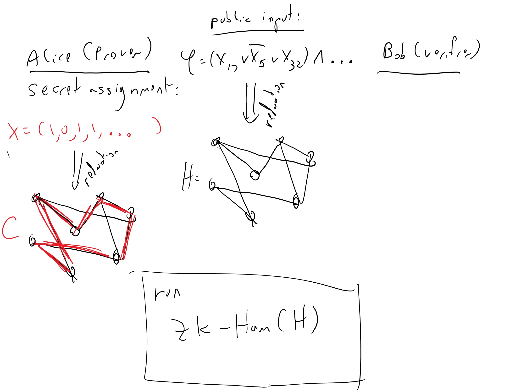
Using the reduction above, we can transform the zero-knowledge proof for Hamiltonicity into a zero knowledge proof for every \(F\in \ensuremath{\mathit{NP}}\). Specifically, to prove that \(F(x)=1\), the verifier and prover will use the following system (see also Figure 13.1).

1. Public input: \(x\). Prover’s private input: \(y\) such that \(V_F(x,y)=1\).

2. Verifier and prover will compute \(G=r(x)\). Prover will compute \(C=r_{Encode}(x,y)\).

3. Verifier and prove run the Hamiltonicity zero knowledge protocol, with public input \(G\) and prover’s private input \(C\). The verifier’s output is the output in this protocol.

This means that for every other NP language \(L\), we can use the reduction from \(L\) to Hamiltonicity combined with protocol ZK-Ham to give a zero knowledge proof system for \(L\). In particular this means that we can have zero knowledge proofs for the following languages:

• The language of numbers \(m\) such that there exists a prime \(p\) dividing \(m\) whose remainder modulo \(10\) is \(7\).

• The language of tuples \(X,e,c_1,\ldots,c_n\) such that \(c_i\) is an encryption of a number \(x_i\) with \(\sum x_i = X\). (This is essentially what we needed in the voting example above).

• For every efficient function \(G\), the language of pairs \(x,y\) such that there exists some input \(r\) satisfying \(y=G(x\|r)\). (This is what we often need in the “protocol compiling” applications to show that a particular output was produced by the correct program \(G\) on public input \(x\) and private input \(r\).)

Parallel repetition and turning zero knowledge proofs to signatures.

While we talked about amplifying zero knowledge proofs by running them \(n\) times one after the other, one could also imagine running the \(n\) copies in parallel. It is not trivial that we get the same benefit of reducing the error to \(2^{-n}\) but it turns out that we do in the cases we are interested in here. Unfortunately, zero knowledge is not necessarily preserved. It’s an important open problem whether zero knowledge is preserved for the ZK-Ham protocol mentioned above.
However, Fiat and Shamir showed that in protocols (such as the ones we showed here) where the verifier only sends random bits, then if we replaced this verifier by a random function, then both soundness and zero knowledge are preserved. This suggests a non-interactive version of these protocols in the random oracle model, and this is indeed widely used. Schnorr designed signatures based on this non interactive version.

“Bonus features” of zero knowledge

The following properties of zero knowledge systems are used in the literature. We might cover some in class, but mention them here. These are covered in Chapter 20 of Boneh-Shoup.

• Proof of knowledge - it can be shown that the proof above of Hamiltonicity yields more than soundness. We can “extract” from a prover startegy that succeeds in convincing the verifier that \(G\) is Hamiltonian with probability larger than 1/2 an actual Hamiltonian cycle. This means that the prover didn’t just convince the verifier that there exists a Hamiltonian cycle in the graph \(G\) but also that the prover “knows” it. This notion is known as a “proof of knowledge”.

• Arguments - if a proof system only satisfies the soundness condition with respect to polynomial-time provers, then it is called an argument system.

• Succinct proofs - proofs that \(F(x)=1\) where total communication is a fixed polynomial in \(n\) independently of the time to verify \(F\).

Combining succinct zero-knowledge proofs with the Fiat-Shamir heuristic for non-interactivity leads to the notion of zero-knowledge succinct arguments or ZK-SNARG. If these also satisfy a “proof of knowledge” property then they are called ZK-SNARKs. These have recently been of great interest for crypto-currencies. See lectures 16-18 in Stanford CS 251, as well as this blog post.

Comments

Comments are posted on the GitHub repository using the utteranc.es app. A GitHub login is required to comment. If you don't want to authorize the app to post on your behalf, you can also comment directly on the GitHub issue for this page.

Compiled on 11/17/2021 22:36:40

Copyright 2021, Boaz Barak.
This work is licensed under a Creative Commons Attribution-NonCommercial-NoDerivatives 4.0 International License.

Produced using pandoc and panflute with templates derived from gitbook and bookdown.