See any bugs/typos/confusing explanations? Open a GitHub issue. You can also comment below
★ See also the PDF version of this chapter (better formatting/references) ★
Introduction
Additional reading: Chapters 1 and 2 of Katz-Lindell book. Sections 2.1 (Introduction) and 2.2 (Shannon ciphers and perfect security) in the Boneh Shoup book. 1
Ever since people started to communicate, there were some messages that they wanted kept secret. Thus cryptography has an old though arguably undistinguished history. For a long time cryptography shared similar features with Alchemy as a domain in which many otherwise smart people would be drawn into making fatal mistakes. Indeed, the history of cryptography is littered with the figurative corpses of cryptosystems believed secure and then broken, and sometimes with the actual corpses of those who have mistakenly placed their faith in these cryptosystems. The definitive text on the history of cryptography is David Kahn’s “The Codebreakers”, whose title already hints at the ultimate fate of most cryptosystems.2 (See also “The Code Book” by Simon Singh.)
We recount below just a few stories to get a feel for this field. But before we do so, we should introduce the cast of characters. The basic setting of “encryption” or “secret writing” is the following: one person, whom we will call Alice, wishes to send another person, whom we will call Bob, a secret message. Since Alice and Bob are not in the same room (perhaps because Alice is imprisoned in a castle by her cousin the queen of England), they cannot communicate directly and need to send their message in writing. Alas, there is a third person, whom we will call Eve, that can see their message. Therefore Alice needs to find a way to encode or encrypt the message so that only Bob (and not Eve) will be able to understand it.
Some history
In 1587, Mary the queen of Scots, and heir to the throne of England, wanted to arrange the assassination of her cousin, queen Elisabeth I of England, so that she could ascend to the throne and finally escape the house arrest under which she had been for the last 18 years. As part of this complicated plot, she sent a coded letter to Sir Anthony Babington.
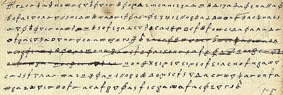
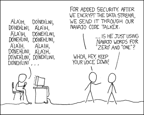
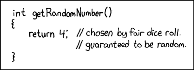
Mary used what’s known as a substitution cipher where each letter is transformed into a different obscure symbol (see Figure 1.1). At a first look, such a letter might seem rather inscrutable- a meaningless sequence of strange symbols. However, after some thought, one might recognize that these symbols repeat several times and moreover that different symbols repeat with different frequencies. Now it doesn’t take a large leap of faith to assume that perhaps each symbol corresponds to a different letter and the more frequent symbols correspond to letters that occur in the alphabet with higher frequency. From this observation, there is a short gap to completely breaking the cipher, which was in fact done by queen Elisabeth’s spies who used the decoded letters to learn of all the co-conspirators and to convict queen Mary of treason, a crime for which she was executed. Trusting in superficial security measures (such as using “inscrutable” symbols) is a trap that users of cryptography have been falling into again and again over the years. (As in many things, this is the subject of a great XKCD cartoon, see Figure 1.2.)
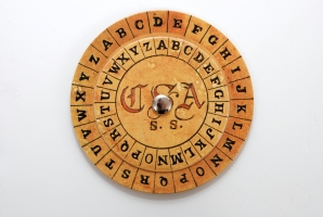
The Vigenère cipher is named after Blaise de Vigenère who described it in a book in 1586 (though it was invented earlier by Bellaso). The idea is to use a collection of substitution ciphers - if there are \(n\) different ciphers then the first letter of the plaintext is encoded with the first cipher, the second with the second cipher, the \(n^{th}\) with the \(n^{th}\) cipher, and then the \(n+1^{st}\) letter is again encoded with the first cipher. The key is usually a word or a phrase of \(n\) letters, and the \(i^{th}\) substitution cipher is obtained by shifting each letter \(k_i\) positions in the alphabet. This “flattens” the frequencies and makes it much harder to do frequency analysis, which is why this cipher was considered “unbreakable” for 300+ years and got the nickname “le chiffre indéchiffrable” (“the unbreakable cipher”). Nevertheless, Charles Babbage cracked the Vigenère cipher in 1854 (though he did not publish it). In 1863 Friedrich Kasiski broke the cipher and published the result. The idea is that once you guess the length of the cipher, you can reduce the task to breaking a simple substitution cipher which can be done via frequency analysis (can you see why?). Confederate generals used Vigenère regularly during the civil war, and their messages were routinely cryptanalyzed by Union officers.
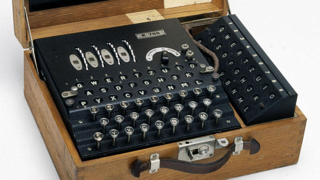
The Enigma cipher was a mechanical cipher (looking like a typewriter, see Figure 1.5) where each letter typed would get mapped into a different letter depending on the (rather complicated) key and current state of the machine which had several rotors that rotated at different paces. An identically wired machine at the other end could be used to decrypt. Just as many ciphers in history, this has also been believed by the Germans to be “impossible to break” and even quite late in the war they refused to believe it was broken despite mounting evidence to that effect. (In fact, some German generals refused to believe it was broken even after the war.) Breaking Enigma was an heroic effort which was initiated by the Poles and then completed by the British at Bletchley Park, with Alan Turing (of the Turing machines) playing a key role. As part of this effort the Brits built arguably the world’s first large scale mechanical computation devices (though they looked more similar to washing machines than to iPhones). They were also helped along the way by some quirks and errors of the German operators. For example, the fact that their messages ended with “Heil Hitler” turned out to be quite useful.
Here is one entertaining anecdote: the Enigma machine would never map a letter to itself. In March 1941, Mavis Batey, a cryptanalyst at Bletchley Park received a very long message that she tried to decrypt. She then noticed a curious property— the message did not contain the letter “L”.3 She realized that the probability that no “L”’s appeared in the message is too small for this to happen by chance. Hence she surmised that the original message must have been composed only of L’s. That is, it must have been the case that the operator, perhaps to test the machine, have simply sent out a message where he repeatedly pressed the letter “L”. This observation helped her decode the next message, which helped inform of a planned Italian attack and secure a resounding British victory in what became known as “the Battle of Cape Matapan”. Mavis also helped break another Enigma machine. Using the information she provided, the Brits were able to feed the Germans with the false information that the main allied invasion would take place in Pas de Calais rather than on Normandy.
In the words of General Eisenhower, the intelligence from Bletchley park was of “priceless value”. It made a huge difference for the Allied war effort, thereby shortening World War II and saving millions of lives. See also this interview with Sir Harry Hinsley.
Defining encryptions
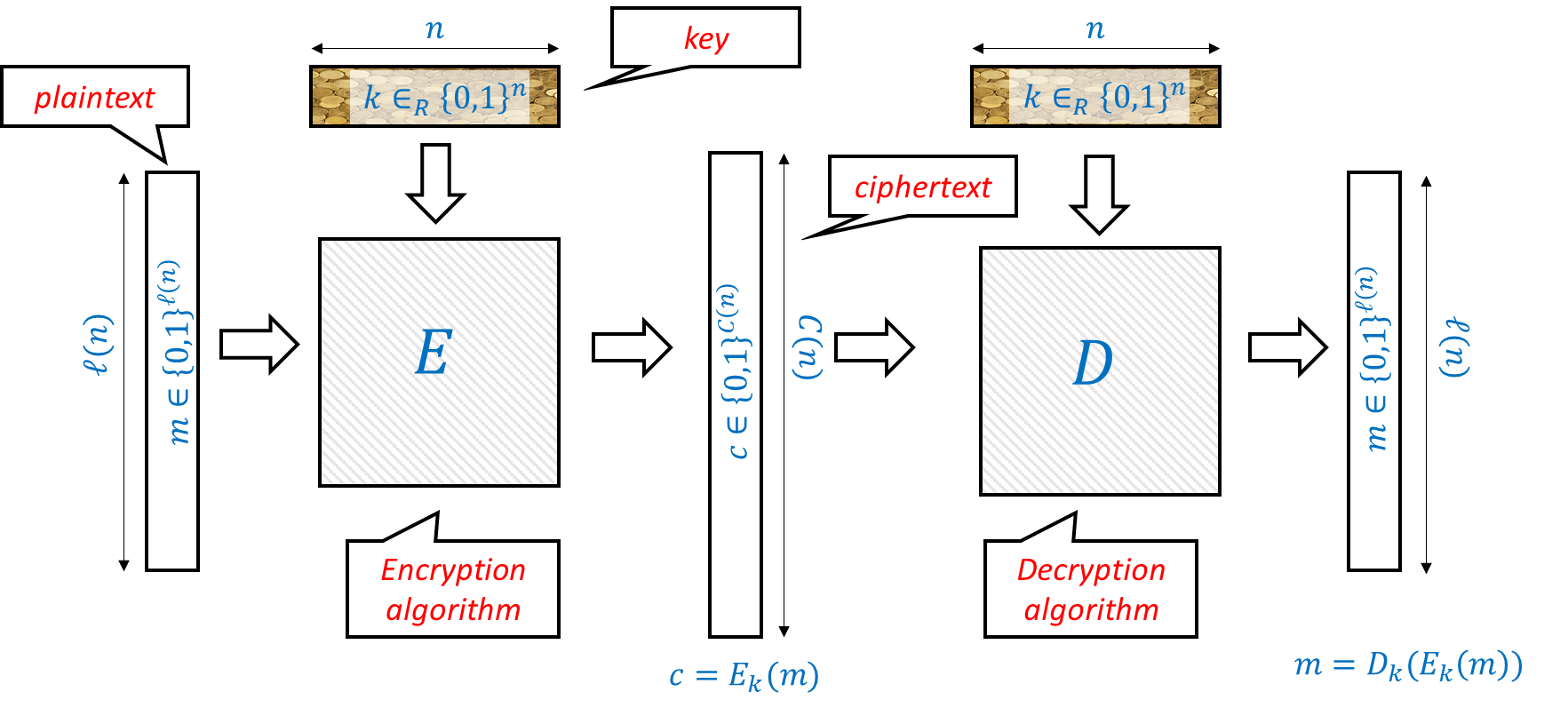
Many of the troubles that cryptosystem designers faced over history (and still face!) can be attributed to not properly defining or understanding what the goals they want to achieve are in the first place. We now turn to actually defining what is an encryption scheme. Clearly we can encode every message as a string of bits, i.e., an element of \(\{0,1\}^\ell\) for some \(\ell\). Similarly, we can encode the key as a string of bits as well, i.e., an element of \(\{0,1\}^n\) for some \(n\). Thus, we can think of an encryption scheme as composed of two functions. The encryption function \(E\) maps a secret key \(k \in \{0,1\}^n\) and a message (known also as plaintext) \(m\in \{0,1\}^\ell\) into a ciphertext \(c \in \{0,1\}^L\) for some \(L\). We write this as \(c = E_k(m)\). The decryption function \(D\) does the reverse operation, mapping the secret key \(k\) and the ciphertext \(c\) back into the plaintext message \(m\), which we write as \(m = D_k(c)\). The basic equation is that if we use the same key for encryption and decryption, then we should get the same message back. That is, for every \(k \in \{0,1\}^n\) and \(m\in \{0,1\}^\ell\),
This motivates the following definition which attempts to capture what it means for an encryption scheme to be valid or “make sense”, regardless of whether or not it is secure:
Let \(\ell:\N \rightarrow \N\) and \(C:\N \rightarrow \N\) be two functions mapping natural numbers to natural numbers. A pair of polynomial-time computable functions \((E,D)\) mapping strings to strings is a valid private key encryption scheme (or encryption scheme for short) with plaintext length function \(\ell(\cdot)\) and ciphertext length function \(C(\cdot)\) if for every \(n\in \N\), \(k\in \{0,1\}^n\) and \(m \in \{0,1\}^{\ell(n)}\), \(|E_k(m)|= C(n)\) and
We will often write the first input (i.e., the key) to the encryption and decryption as a subscript and so can write Equation 1.1 also as \(D_k(E_k(m))=m\).
The validity condition implies that for any fixed \(k\), the map \(m \mapsto E_k(m)\) is one to one (can you see why?) and hence the ciphertext length is always at least the plaintext length. Thus we typically focus on the plaintext length as the quantity to optimize in an encryption scheme. The larger \(\ell(n)\) is, the better the scheme, since it means we need a shorter secret key to protect messages of the same length.
A note on notation: We will always use \(i,j,\ell,n\) to denote natural numbers.
The number \(n\) will often denote the length of our secret key. The length of the key (or another closely related number) is often known as the security parameter in the literature. Katz-Lindell also uses \(n\) to denote this parameter, while Boneh-Shoup and Rosulek use \(\lambda\) for it. (Some texts also use the Greek letter \(\kappa\) for the same parameter.) We chose to denote the security parameter by \(n\) as to correspond with the standard algorithmic notation for input length (as in \(O(n)\) or \(O(n^2)\) time algorithms).
We often use \(\ell\) to denote the length of the message, sometimes also known as “block length” since longer messages are simply chopped into “blocks” of length \(\ell\) and also appropriately padded.
We will use \(k\) to denote the secret key, \(m\) to denote the secret plaintext message, and \(c\) to denote the encrypted ciphertext. Note that \(k,m,c\) are not numbers but rather bit strings of lengths \(n,\ell(n),C(n)\) respectively. We will also sometimes use \(x\) and \(y\) to denote strings, and so sometimes use \(x\) as the plaintext and \(y\) as the ciphertext. In general, while we try to reserve variable names for particular purposes, cryptography uses so many concepts that it would sometimes need to “reuse” the same letter for different purposes.
For simplicity, we denote the space of possible keys as \(\{0,1\}^n\) and the space of possible messages as \(\{0,1\}^\ell\) for \(\ell=\ell(n)\). Boneh-Shoup uses a more general notation of \(\mathcal{K}\) for the space of all possible keys and \(\mathcal{M}\) for the space of all possible messages. This does not make much difference since we can represent every discrete object such as a key or message as a binary string. (One difference is that in principle the space of all possible messages could include messages of unbounded length, though in such a case what is done in both theory and practice is to break these up into finite-size blocks and encrypt one block at a time.)
Defining security of encryption
Definition 1.1 says nothing about security and does not rule out trivial “encryption” schemes such as the scheme \(E_k(m) = m\) that simply outputs the plaintext as is. Defining security is tricky, and we’ll take it one step at a time, but let’s start by pondering what is secret and what is not. A priori we are thinking of an attacker Eve that simply sees the ciphertext \(c=E_k(m)\) and does not know anything on how it was generated. So, it does not know the details of \(E\) and \(D\), and certainly does not know the secret key \(k\). However, many of the troubles past cryptosystems went through were caused by them relying on “security through obscurity”— trusting that the fact their methods are not known to their enemy will protect them from being broken. This is a faulty assumption - if you reuse a method again and again (even with a different key each time) then eventually your adversaries will figure out what you are doing. And if Alice and Bob meet frequently in a secure location to decide on a new method, they might as well take the opportunity to exchange their secret messages…
These considerations led Auguste Kerckhoffs in 1883 to state the following principle:
A cryptosystem should be secure even if everything about the system, except the key, is public knowledge.4
Why is it OK to assume the key is secret and not the algorithm? Because we can always choose a fresh key. But of course that won’t help us much if our key is “1234” or “passw0rd!”. In fact, if you use any deterministic algorithm to choose the key then eventually your adversary will figure this out. Therefore for security we must choose the key at random and can restate Kerckhoffs’s principle as follows:
There is no secrecy without randomness
This is such a crucial point that is worth repeating:
There is no secrecy without randomness
At the heart of every cryptographic scheme there is a secret key, and the secret key is always chosen at random. A corollary of that is that to understand cryptography, you need to know some probability theory. Fortunately, we don’t need much of probability- only probability over finite spaces, and basic notions such as expectation, variance, concentration and the union bound suffice for most of we need. In fact, understanding the following two statements will already get you much of what you need for cryptography:
For every fixed string \(x\in\{0,1\}^n\), if you toss a coin \(n\) times, the probability that the heads/tails pattern will be exactly \(x\) is \(2^{-n}\).
A probability of \(2^{-128}\) is really really small.
Generating randomness in actual cryptographic systems
How do we actually get random bits in actual systems? The main idea is to use a two stage approach. First we need to get some data that is unpredictable from the point of view of an attacker on our system. Some sources for this could be measuring latency on the network or hard drives (getting harder with solid state disk), user keyboard and mouse movement patterns (problematic when you need fresh randomness at boot time ), clock drift and more, there are some other sources including audio, video, and network. All of these can be problematic, especially for servers or virtual machines, and so hardware based random number generators based on phenomena such as thermal noise or nuclear decay are becoming more popular. Once we have some data \(X\) that is unpredictable, we need to estimate the entropy in it. You can roughly imagine that \(X\) has \(k\) bits of entropy if the probability that an attacker can guess \(X\) is at most \(2^{-k}\). People then use a hash function (an object we’ll talk about more later) to map \(X\) into a string of length \(k\) which is then hopefully distributed (close to) uniformly at random. All of this process, and especially understanding the amount of information an attacker may have on the entropy sources, is a bit of a dark art and indeed a number of attacks on cryptographic systems were actually enabled by weak generation of randomness. Here are a few examples.
One of the first attacks was on the SSL implementation of Netscape (the browser at the time). Netscape used the following “unpredictable” information— the time of day and a process ID both of which turned out to be quite predictable (who knew attackers have clocks too?). Netscape tried to protect its security through “security through obscurity” by not releasing the source code for their pseudorandom generator, but it was reverse engineered by Ian Goldberg and David Wagner (Ph.D students at the time) who demonstrated this attack.
In 2006 a programmer removed a line of code from the procedure to generate entropy in OpenSSL package distributed by Debian since it caused a warning in some automatic verification code. As a result for two years (until this was discovered) all the randomness generated by this procedure used only the process ID as an “unpredictable” source. This means that all communication done by users in that period is fairly easily breakable (and in particular, if some entities recorded that communication they could break it also retroactively). This caused a huge headache and a worldwide regeneration of keys, though it is believed that many of the weak keys are still used. See XKCD’s take on that incident.
In 2012 two separate teams of researchers scanned a large number of RSA keys on the web and found out that about 4 percent of them are easy to break. The main issue were devices such as routers, internet-connected printers and such. These devices sometimes run variants of Linux- a desktop operating system- but without a hard drive, mouse or keyboard, they don’t have access to many of the entropy sources that desktops have. Coupled with some good old fashioned ignorance of cryptography and software bugs, this led to many keys that are downright trivial to break, see this blog post and this web page for more details.
After the entropy is collected and then “purified” or “extracted” to a uniformly random string that is, say, a few hundred bits long, we often need to “expand” it into a longer string that is also uniform (or at least looks like that for all practical purposes). We will discuss how to go about that in the next lecture. This step has its weaknesses too, and in particular the Snowden documents, combined with observations of Shumow and Ferguson, strongly suggest that the NSA has deliberately inserted a trapdoor in one of the pseudorandom generators published by the National Institute of Standards and Technologies (NIST). Fortunately, this generator wasn’t widely adopted, but apparently the NSA did pay 10 million dollars to RSA security so the latter would make this generator their default option in their products.
Defining the secrecy requirement.
Defining the secrecy requirement for an encryption is not simple. Over the course of history, many smart people got it wrong and convinced themselves that ciphers were impossible to break. The first person to truly ask the question in a rigorous way was Claude Shannon in 1945 (though a partial version of his manuscript was only declassified in 1949). Simply by asking this question, he made an enormous contribution to the science of cryptography and practical security. We now will try to examine how one might answer it.
Let me warn you ahead of time that we are going to insist on a mathematically precise definition of security. That means that the definition must capture security in all cases, and the existence of a single counterexample, no matter how “silly”, would make us rule out a candidate definition. This exercise of coming up with “silly” counterexamples might seem, well, silly. But in fact it is this method that has led Shannon to formulate his theory of secrecy, which (after much followup work) eventually revolutionized cryptography, and brought this science to a new age where Edgar Allan Poe’s maxim no longer holds, and we are able to design ciphers which human (or even nonhuman) ingenuity cannot break.
The most natural way to attack an encryption is for Eve to guess all possible keys. In many encryption schemes this number is enormous and this attack is completely infeasible. For example, the theoretical number of possibilities in the Enigma cipher was about \(10^{113}\) which roughly means that even if we filled the milky way galaxy with computers operating at light speed, the sun would still die out before it finished examining all the possibilities.5 One can understand why the Germans thought it was impossible to break. (Note that despite the number of possibilities being so enormous, such a key can still be easily specified and shared between Alice and Bob by writing down \(113\) digits on a piece of paper.) Ray Miller of the NSA had calculated that, in the way the Germans used the machine, the number of possibilities was “only” \(10^{23}\), but this is still extremely difficult to pull off even today, and many orders of magnitudes above the computational powers during the WW-II era. Thus clearly, it is sometimes possible to break an encryption without trying all possibilities. A corollary is that having a huge number of key combinations does not guarantee security, as an attacker might find a shortcut (as the allies did for Enigma) and recover the key without trying all options.
Since it is possible to recover the key with some tiny probability (e.g. by guessing it at random), perhaps one way to define security of an encryption scheme is that an attacker can never recover the key with probability significantly higher than that. Here is an attempt at such a definition:
An encryption scheme \((E,D)\) is \(n\)-secure if no matter what method Eve employs, the probability that she can recover the true key \(k\) from the ciphertext \(c\) is at most \(2^{-n}\).
When you see a mathematical definition that attempts to model some real-life phenomenon such as security, you should pause and ask yourself:
Do I understand mathematically what the definition is stating?
Is it a reasonable way to capture the real life phenomenon we are discussing?
One way to answer question 2 is to try to think of both examples of objects that satisfy the definition and examples of objects that violate it, and see if this conforms to your intuition about whether these objects display the phenomenon we are trying to capture. Try to do this for Definition 1.3
You might wonder if Definition 1.3 is not too strong. After all how are we going to ever prove that Eve cannot recover the secret key no matter what she does? Edgar Allan Poe would say that there can always be a method that we overlooked. However, in fact this definition is too weak! Consider the following encryption: the secret key \(k\) is chosen at random in \(\{0,1\}^n\) but our encryption scheme simply ignores it and lets \(E_k(m)=m\) and \(D_k(c)=c\). This is a valid encryption since \(D_k(E_k(m))=m\), but is of course completely insecure as we are simply outputting the plaintext in the clear. Yet, no matter what Eve does, if she only sees \(c\) and not \(k\), there is no way she can guess the true value of \(k\) with probability better than \(2^{-n}\), since it was chosen completely at random and she gets no information about it. Formally, one can prove the following result:
Let \((E,D)\) be the encryption scheme above. For every function \(Eve:\{0,1\}^\ell\rightarrow \{0,1\}^n\) and for every \(m\in \{0,1\}^\ell\), the probability that \(Eve(E_k(m))=k\) is exactly \(2^{-n}\).
This follows because \(E_k(m)=m\) and hence \(Eve(E_k(m))=Eve(m)\) which is some fixed value \(k'\in\{0,1\}^n\) that is independent of \(k\). Hence the probability that \(k=k'\) is \(2^{-n}\). QED
The math behind the above argument is very simple, yet I urge you to read and re-read the last two paragraphs until you are sure that you completely understand why this encryption is in fact secure according to the above definition. This is a “toy example” of the kind of reasoning that we will be employing constantly throughout this course, and you want to make sure that you follow it.
So, Lemma 1.4 is true, but one might question its meaning. Clearly this silly example was not what we meant when stating this definition. However, as mentioned above, we are not willing to ignore even silly examples and must amend the definition to rule them out. One obvious objection is that we don’t care about hiding the key- it is the message that we are trying to keep secret. This suggests the next attempt:
An encryption scheme \((E,D)\) is \(n\)-secure if for every message \(m\) no matter what method Eve employs, the probability that she can recover \(m\) from the ciphertext \(c=E_k(m)\) is at most \(2^{-n}\).
Now this seems like it captures our intended meaning. But remember that we are being anal, and truly insist that the definition holds as stated, namely that for every plaintext message \(m\) and every function \(Eve:\{0,1\}^C\rightarrow\{0,1\}^\ell\), the probability over the choice of \(k\) that \(Eve(E_k(m))=m\) is at most \(2^{-n}\). But now we see that this is clearly impossible. After all, this is supposed to work for every message \(m\) and every function \(Eve\), but clearly if \(m\) is the all-zeroes message \(0^\ell\) and \(Eve\) is the function that ignores its input and simply outputs \(0^\ell\), then it will hold that \(Eve(E_k(m))=m\) with probability one.
So, if before the definition was too weak, the new definition is too strong and is impossible to achieve. The problem is that of course we could guess a fixed message with probability one, so perhaps we could try to consider a definition with a random message. That is:
An encryption scheme \((E,D)\) is \(n\)-secure if no matter what method Eve employs, if \(m\) is chosen at random from \(\{0,1\}^\ell\), the probability that she can recover \(m\) from the ciphertext \(c=E_k(m)\) is at most \(2^{-n}\).
This weakened definition can in fact be achieved, but we have again weakened it too much. Consider an encryption that hides the last \(\ell/2\) bits of the message, but completely reveals the first \(\ell/2\) bits. The probability of guessing a random message is \(2^{-\ell/2}\), and so such a scheme would be “\(\ell/2\) secure” per Definition 1.6 but this is still a scheme that you would not want to use. The point is that in practice we don’t encrypt random messages— our messages might be in English, might have common headers, and might have even more structures based on the context. In fact, it may be that the message is either “Yes” or “No” (or perhaps either “Attack today” or “Attack tomorrow”) but we want to make sure Eve doesn’t learn which one it is. So, using an encryption scheme that reveals the first half of the message (or frankly even only the first bit) is unacceptable.
Perfect Secrecy
So far all of our attempts at definitions oscillated between being too strong (and hence impossible) or too weak (and hence not guaranteeing actual security). The key insight of Shannon was that in a secure encryption scheme the ciphertext should not reveal any additional information about the plaintext. So, if for example it was a priori possible for Eve to guess the plaintext with some probability \(1/k\) (e.g., because there were only \(k\) possibilities for it) then she should not be able to guess it with higher probability after seeing the ciphertext. This can be formalized as follows:
An encryption scheme \((E,D)\) is perfectly secret if there for every set \(M\subseteq\{0,1\}^\ell\) of plaintexts, and for every strategy used by Eve, if we choose at random \(m\in M\) and a random key \(k\in\{0,1\}^n\), then the probability that Eve guesses \(m\) after seeing \(E_k(m)\) is at most \(1/|M|\).
In particular, if we encrypt either “Yes” or “No” with probability \(1/2\), then Eve won’t be able to guess which one it is with probability better than half. In fact, that turns out to be the heart of the matter:
An encryption scheme \((E,D)\) is perfectly secret if and only if for every two distinct plaintexts \(\{m_0,m_1\} \subseteq \{0,1\}^\ell\) and every strategy used by Eve, if we choose at random \(b\in\{0,1\}\) and a random key \(k\in\{0,1\}^n\), then the probability that Eve guesses \(m_b\) after seeing \(E_k(m_b)\) is at most \(1/2\).
The “only if” direction is obvious— this condition is a special case of the perfect secrecy condition for a set \(M\) of size \(2\).
The “if” direction is trickier. We will use a proof by contradiction. We need to show that if there is some set \(M\) (of size possibly much larger than \(2\)) and some strategy for Eve to guess (based on the ciphertext) a plaintext chosen from \(M\) with probability larger than \(1/|M|\), then there is also some set \(M'\) of size two and a strategy \(Eve'\) for Eve to guess a plaintext chosen from \(M'\) with probability larger than \(1/2\).
Let’s fix the message \(m_0\) to be the all zeroes message and pick \(m_1\) at random in \(M\). Under our assumption, it holds that for random key \(k\) and message \(m_1\in M\), On the other hand, for every choice of \(k\), \(m'= Eve(E_k(m_0))\) is a fixed string independent on the choice of \(m_1\), and so if we pick \(m_1\) at random in \(M\), then the probability that \(m_1=m'\) is at most \(1/|M|\), or in other words
We can also write Equation 1.2 and Equation 1.3 as
In particular, by the averaging argument (the argument that if the average of numbers is larger than \(\alpha\) then one of the numbers is larger than \(\alpha\)) there must exist \(m_1 \in M\) satisfying
But this can be turned into an attacker \(Eve'\) such that for \(b \leftarrow_R \{0,1\}\). the probability that \(Eve'(E_k(m_b))=m_b\) is larger than \(1/2\). Indeed, we can define \(Eve'(c)\) to output \(m_1\) if \(Eve(c)=m_1\) and otherwise output a random message in \(\{ m_0 , m_1 \}\). The probability that \(Eve'(y)\) equals \(m_1\) is higher when \(c=E_k(m_1)\) than when \(c=E_k(m_0)\), and since \(Eve'\) outputs either \(m_0\) or \(m_1\), this means that the probability that \(Eve'(E_k(m_b))=m_b\) is larger than \(1/2\). (Can you see why?)
The proof of Theorem 1.8 is not trivial, and is worth reading again and making sure you understand it. An excellent exercise, which I urge you to pause and do now is to prove the following: \((E,D)\) is perfectly secret if for every plaintexts \(m,m' \in \{0,1\}^\ell\), the two random variables \(\{ E_k(m) \}\) and \(\{ E_{k'}(m') \}\) (for randomly chosen keys \(k\) and \(k'\)) have precisely the same distribution.
Prove that a valid encryption scheme \((E,D)\) with plaintext length \(\ell(\cdot)\) is perfectly secret if and only if for every \(n\in \N\) and plaintexts \(m,m' \in \{0,1\}^{\ell(n)}\), the following two distributions \(Y\) and \(Y'\) over \(\{0,1\}^*\) are identical:
\(Y\) is obtained by sampling \(k\leftarrow_R \{0,1\}^n\) and outputting \(E_k(m)\).
\(Y'\) is obtained by sampling \(k\leftarrow_R \{0,1\}^n\) and outputting \(E_k(m')\).
We only sketch the proof. The condition in the exercise is equivalent to perfect secrecy with \(|M|=2\). For every \(M = \{ m,m' \}\), if \(Y\) and \(Y'\) are identical then clearly for every \(Eve\) and possible output \(y\), \(\Pr[ Eve(E_k(m))=y] = \Pr[ Eve(E_k(m'))=y]\) since these correspond applying \(Eve\) on the same distribution \(Y=Y'\). On the other hand, if \(Y\) and \(Y'\) are not identical then there must exist some ciphertext \(c^*\) such that \(\Pr[ Y=c^*] > \Pr[ Y'=c^*]\) (or vice versa). The adversary that on input \(c\) guesses that \(c\) is an encryption of \(m\) if \(c=c^*\) and otherwise tosses a coin will have some advantage over \(1/2\) in distinguishing an encryption of \(m\) from an encryption of \(m'\).
We summarize the equivalent definitions of perfect secrecy in the following theorem, whose (omitted) proof follows from Theorem 1.8 and Solved Exercise 1.1 as well as similar proof ideas.
Let \((E,D)\) be a valid encryption scheme with message length \(\ell(n)\). Then the following conditions are equivalent:
\((E,D)\) is perfectly secret as per Definition 1.7.
For every pair of messages \(m_0,m_1 \in \{0,1\}^{\ell(n)}\), the distributions \(\{ E_k(m_0) \}_{k \leftarrow_R \{0,1\}^n}\) and \(\{ E_k(m_1) \}_{k \leftarrow_R \{0,1\}^n}\) are identical.
(Two-message security: Eve can’t guess which of one of two messages was encrypted with success better than half.) For every function \(Eve:\{0,1\}^{C(n)} \rightarrow \{0,1\}^{\ell(n)}\) and pair of messages \(m_0,m_1 \in \{0,1\}^{\ell(n)}\),
- (Arbitrary prior security: Eve can’t guess which message was encrypted with success better than her prior information.) For every distribution \(\mathcal{D}\) over \(\{0,1\}^{\ell(n)}\), and \(Eve:\{0,1\}^{C(n)} \rightarrow \{0,1\}^{\ell(n)}\),
where we denote \(\max(\mathcal{D}) = \max_{m^*\in \{0,1\}^{\ell(n)}} \Pr_{m \leftarrow_R \mathcal{D}}[m=m^*]\) to be the largest probability of any element under \(\mathcal{D}\).
Achieving perfect secrecy
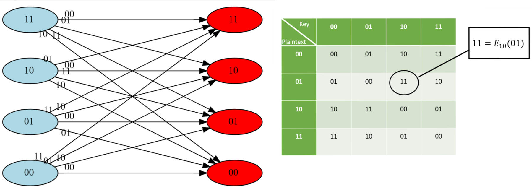
So, perfect secrecy is a natural condition, and does not seem to be too weak for applications, but can it actually be achieved? After all, the condition that two different plaintexts are mapped to the same distribution seems somewhat at odds with the condition that Bob would succeed in decrypting the ciphertexts and find out if the plaintext was in fact \(m\) or \(m'\). It turns out the answer is yes! For example, Figure 1.8 details a perfectly secret encryption for two bits.
In fact, this can be generalized to any number of bits:6
There is a perfectly secret valid encryption scheme \((E,D)\) with \(\ell(n)=n\).
Our scheme is the one-time pad also known as the “Vernam Cipher”, see Figure 1.9. The encryption is exceedingly simple: to encrypt a message \(m\in \{0,1\}^n\) with a key \(k \in \{0,1\}^n\) we simply output \(m \oplus k\) where \(\oplus\) is the bitwise XOR operation that outputs the string corresponding to XORing each coordinate of \(m\) and \(k\).
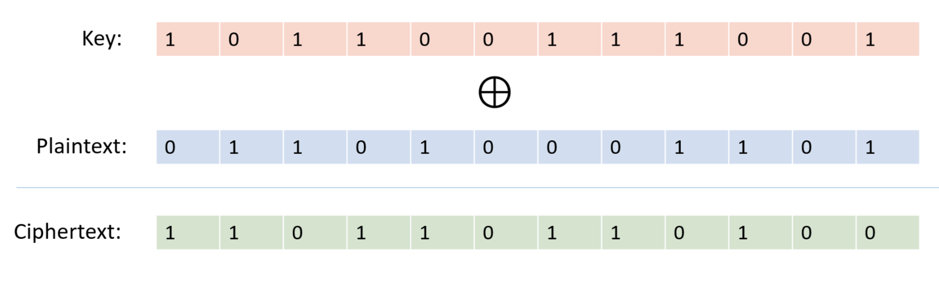
For two binary strings \(a\) and \(b\) of the same length \(n\), we define \(a \oplus b\) to be the string \(c \in \{0,1\}^n\) such that \(c_i = a_i + b_i \mod 2\) for every \(i\in [n]\). The encryption scheme \((E,D)\) is defined as follows: \(E_k(m) = m\oplus k\) and \(D_k(c)= c \oplus k\). By the associative law of addition (which works also modulo two), \(D_k(E_k(m))=(m\oplus k) \oplus k = m \oplus (k \oplus k) = m \oplus 0^n = m\), using the fact that for every bit \(\sigma \in \{0,1\}\), \(\sigma + \sigma \mod 2 = 0\) and \(\sigma + 0 = \sigma \mod 2\). Hence \((E,D)\) form a valid encryption.
To analyze the perfect secrecy property, we claim that for every \(m\in \{0,1\}^n\), the distribution \(Y_m=E_k(m)\) where \(k \leftarrow_R \{0,1\}^n\) is simply the uniform distribution over \(\{0,1\}^n\), and hence in particular the distributions \(Y_{m}\) and \(Y_{m'}\) are identical for every \(m,m' \in \{0,1\}^n\). Indeed, for every particular \(y\in \{0,1\}^n\), the value \(y\) is output by \(Y_m\) if and only if \(y = m \oplus k\) which holds if and only if \(k= m \oplus y\). Since \(k\) is chosen uniformly at random in \(\{0,1\}^n\), the probability that \(k\) happens to equal \(m \oplus y\) is exactly \(2^{-n}\), which means that every string \(y\) is output by \(Y_m\) with probability \(2^{-n}\).
The argument above is quite simple but is worth reading again. To understand why the one-time pad is perfectly secret, it is useful to envision it as a bipartite graph as we’ve done in Figure 1.8. (In fact the encryption scheme of Figure 1.8 is precisely the one-time pad for \(n=2\).) For every \(n\), the one-time pad encryption scheme corresponds to a bipartite graph with \(2^n\) vertices on the “left side” corresponding to the plaintexts in \(\{0,1\}^n\) and \(2^n\) vertices on the “right side” corresponding to the ciphertexts \(\{0,1\}^n\). For every \(x\in \{0,1\}^n\) and \(k\in \{0,1\}^n\), we connect \(x\) to the vertex \(y=E_k(x)\) with an edge that we label with \(k\). One can see that this is the complete bipartite graph, where every vertex on the left is connected to all vertices on the right. In particular this means that for every left vertex \(x\), the distribution on the ciphertexts obtained by taking a random \(k\in \{0,1\}^n\) and going to the neighbor of \(x\) on the edge labeled \(k\) is the uniform distribution over \(\{0,1\}^n\). This ensures the perfect secrecy condition.
Necessity of long keys
So, does Theorem 1.10 give the final word on cryptography, and means that we can all communicate with perfect secrecy and live happily ever after? No it doesn’t. While the one-time pad is efficient, and gives perfect secrecy, it has one glaring disadvantage: to communicate \(n\) bits you need to store a key of length \(n\). In contrast, practically used cryptosystems such as AES-128 have a short key of \(128\) bits (i.e., \(16\) bytes) that can be used to protect terabytes or more of communication! Imagine that we all needed to use the one time pad. If that was the case, then if you had to communicate with \(m\) people, you would have to maintain (securely!) \(m\) huge files that are each as long as the length of the maximum total communication you expect with that person. Imagine that every time you opened an account with Amazon, Google, or any other service, they would need to send you in the mail (ideally with a secure courier) a DVD full of random numbers, and every time you suspected a virus, you’d need to ask all these services for a fresh DVD. This doesn’t sound so appealing.
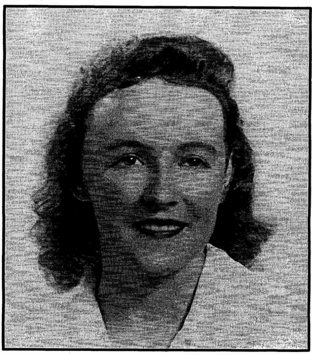
This is not just a theoretical issue. The Soviets have used the one-time pad for their confidential communication since before the 1940’s. In fact, even before Shannon’s work, the U.S. intelligence already knew in 1941 that the one-time pad is in principle “unbreakable” (see page 32 in the Venona document). However, it turned out that the hassle of manufacturing so many keys for all the communication took its toll on the Soviets and they ended up reusing the same keys for more than one message. They did try to use them for completely different receivers in the (false) hope that this wouldn’t be detected. The Venona Project of the U.S. Army was founded in February 1943 by Gene Grabeel (see Figure 1.11), a former home economics teacher from Madison Heights, Virginia and Lt. Leonard Zubko. In October 1943, they had their breakthrough when it was discovered that the Russians were reusing their keys. In the 37 years of its existence, the project has resulted in a treasure chest of intelligence, exposing hundreds of KGB agents and Russian spies in the U.S. and other countries, including Julius Rosenberg, Harry Gold, Klaus Fuchs, Alger Hiss, Harry Dexter White and many others.
Unfortunately it turns out that that such long keys are necessary for perfect secrecy:
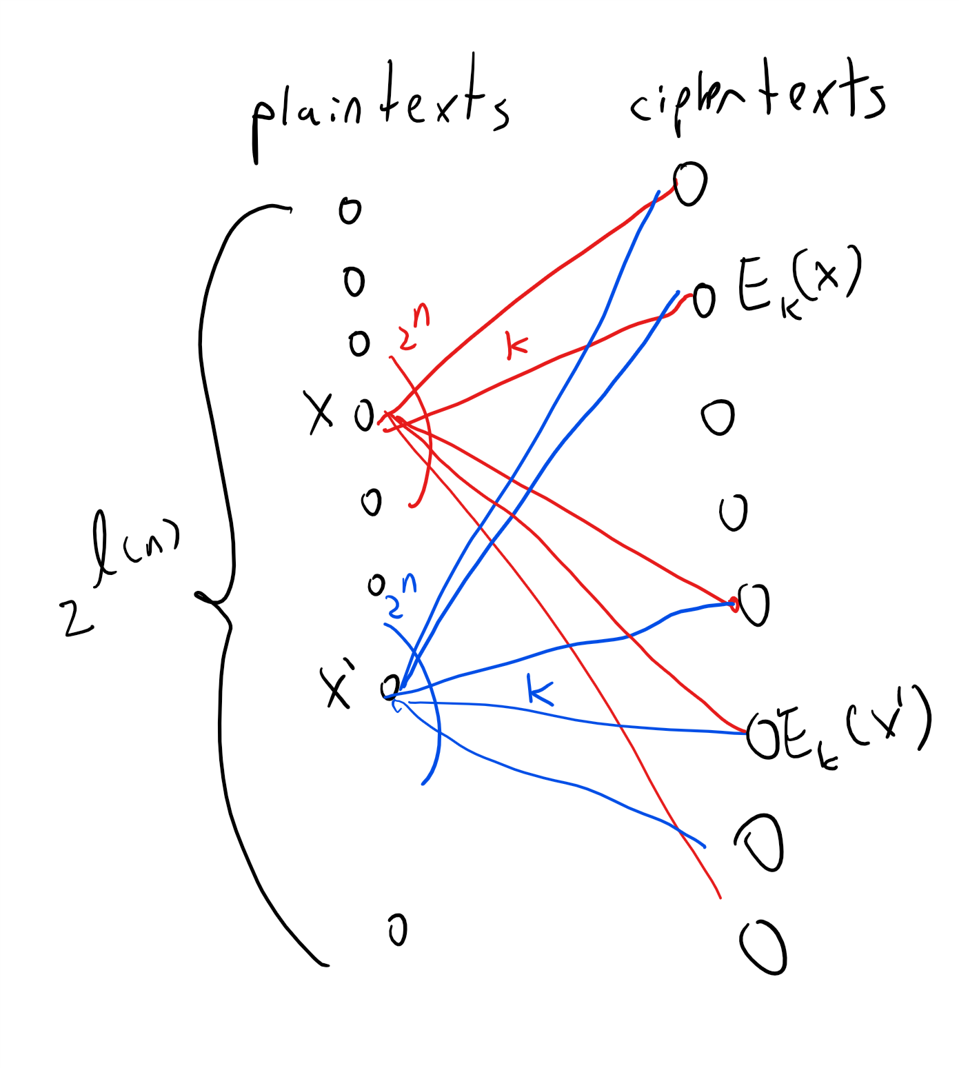
For every perfectly secret encryption scheme \((E,D)\) the length function \(\ell\) satisfies \(\ell(n) \leq n\).
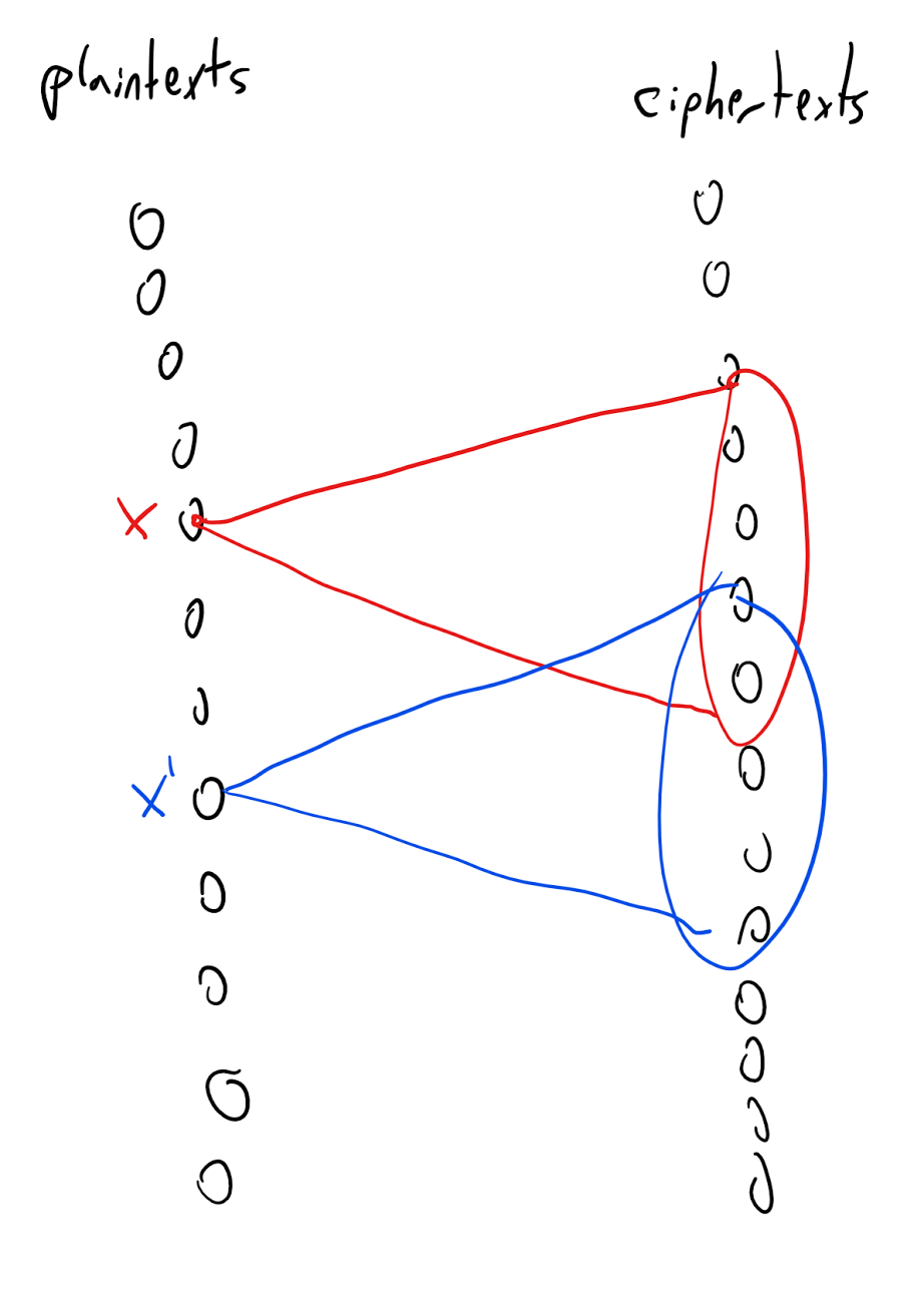
The idea behind the proof is illustrated in Figure 1.12. We define a graph between the plaintexts and ciphertexts, where we put an edge between plaintext \(x\) and ciphertext \(y\) if there is some key \(k\) such that \(y=E_k(x)\). The degree of this graph is at most the number of potential keys. The fact that the degree is smaller than the number of plaintexts (and hence of ciphertexts) implies that there would be two plaintexts \(x\) and \(x'\) with different sets of neighbors, and hence the distribution of a ciphertext corresponding to \(x\) (with a random key) will not be identical to the distribution of a ciphertext corresponding to \(x'\).
Let \(E,D\) be a valid encryption scheme with messages of length \(\ell\) and key of length \(n<\ell\). We will show that \((E,D)\) is not perfectly secret by providing two plaintexts \(x_0,x_1 \in \{0,1\}^\ell\) such that the distributions \(Y_{x_0}\) and \(Y_{x_1}\) are not identical, where \(Y_x\) is the distribution obtained by picking \(k \leftarrow_R \{0,1\}^n\) and outputting \(E_k(x)\).
We choose \(x_0 = 0^\ell\). Let \(S_0 \subseteq \{0,1\}^*\) be the set of all ciphertexts that have nonzero probability of being output in \(Y_{x_0}\). That is, \(S_0=\{ y \;|\; \exists_{k\in \{0,1\}^n} y=E_k(x_0) \}\). Since there are only \(2^n\) keys, we know that \(|S_0| \leq 2^n\).
We will show the following claim:
Claim I: There exists some \(x_1 \in \{0,1\}^\ell\) and \(k\in \{0,1\}^n\) such that \(E_k(x_1) \not\in S_0\).
Claim I implies that the string \(E_k(x_1)\) has positive probability of being output by \(Y_{x_1}\) and zero probability of being output by \(Y_{x_0}\) and hence in particular \(Y_{x_0}\) and \(Y_{x_1}\) are not identical. To prove Claim I, just choose a fixed \(k\in \{0,1\}^n\). By the validity condition, the map \(x \mapsto E_k(x)\) is a one to one map of \(\{0,1\}^\ell\) to \(\{0,1\}^*\) and hence in particular the image of this map which is the set \(I_k = \{ y \;|\; \exists_{x\in \{0,1\}^\ell} y=E_k(x) \}\) has size at least (in fact exactly) \(2^\ell\). Since \(|S_0| \leq 2^n < 2^\ell\), this means that \(|I_k|>|S_0|\) and so in particular there exists some string \(y\) in \(I_k \setminus S_0\). But by the definition of \(I_k\) this means that there is some \(x\in \{0,1\}^\ell\) such that \(E_k(x) \not\in S_0\) which concludes the proof of Claim I and hence of Theorem 1.11.
There is a sense in which both our secrecy and our impossibility results might not be fully convincing, and that is that we did not explicitly consider algorithms that use randomness . For example, maybe Eve can break a perfectly secret encryption if she is not modeled as a deterministic function \(Eve:\{0,1\}^o\rightarrow\{0,1\}^\ell\) but rather a probabilistic process. Similarly, maybe the encryption and decryption functions could be probabilistic processes as well. It turns out that none of those matter.
For the former, note that a probabilistic process can be thought of as a distribution over functions, in the sense that we have a collection of functions \(f_1,...,f_N\) mapping \(\{0,1\}^o\) to \(\{0,1\}^\ell\), and some probabilities \(p_1,\ldots,p_N\) (non-negative numbers summing to \(1\)), so we now think of Eve as selecting the function \(f_i\) with probability \(p_i\). But if none of those functions can give an advantage better than \(1/2\), then neither can this collection (this is related to the averaging principle in probability).
A similar (though more involved) argument shows that the impossibility result showing that the key must be at least as long as the message still holds even if the encryption and decryption algorithms are allowed to be probabilistic processes as well (working this out is a great exercise).
Amplifying success probability
Theorem 1.11 implies that for every encryption scheme \((E,D)\) with \(\ell(n)>n\), there is a pair of messages \(x_0,x_1\) and an attacker \(Eve\) that can distinguish between an encryption of \(x_0\) and an encryption of \(x_1\) with success better than \(1/2\). But perhaps Eve’s success is only marginally better than half, say \(0.50001\)? It turns out that’s not the case. If the message is even somewhat larger than the key, the success of Eve can be very close to \(1\):
Let \((E,D)\) be an encryption scheme with \(\ell(n)=n+t\). Then there is a function \(Eve\) and pair of messages \(x_0,x_1\) such that
As in the proof of Theorem 1.11, let \(\ell=\ell(n)\) and let \(x_0 = 0^\ell\) and \(S_0 = \{ E_k(x_0) : k\in \{0,1\}^n \}\) be the set of size at most \(2^n\) of all ciphertexts corresponding to \(x_0\). We claim that
We show this by arguing that this bound holds for every fixed \(k\), when we take the probability over \(x\), and so in particular it holds also for random \(k\). Indeed, for every fixed \(k\), the map \(x \mapsto E_k(x)\) is a one-to-one map, and so the distribution of \(E_k(x)\) for random \(x\in \{0,1\}^\ell\) is uniform over some set \(T_k\) of size \(2^{n+t}\). For every \(k\), the probability over \(x\) that \(E_k(x) \in S_0\) is equal to
Now, for every \(x\), define \(p_x\) to be \(\Pr_{k \leftarrow_R \{0,1\}^n}[ E_k(x) \in S_0]\). By Equation 1.5, the expectation of \(p_x\) over random \(x \leftarrow_R \{0,1\}^n\) is at most \(2^{-t}\) and so in particular by the averaging argument there exists some \(x_1\) such that \(p_{x_1} \leq 2^{-t}\). Yet that means that the following adversary \(Eve\) will be able to distinguish between an encryption of \(x_0\) and an encryption of \(x_1\) with probability at least \(1-2^{-t-1}\):
Input: A ciphertext \(y\in \{0,1\}^*\)
Operation: If \(y\in S_0\), output \(x_0\), otherwise output \(x_1\).
The probability that \(Eve(E_k(x_0))=x_0\) is equal to \(1\), while the probability that \(Eve(E_k(x_1))=x_1\) is equal to \(1-p_{x_1} \geq 1- 2^{-t}\). Hence the overall probability of \(Eve\) guessing correctly is
Bibliographical notes
Much of this text is shared with my Introduction to Theoretical Computer Science textbook.
Shannon’s manuscript was written in 1945 but was classified, and a partial version was only published in 1949. Still it has revolutionized cryptography, and is the forerunner to much of what followed.
The Venona project’s history is described in this document. Aside from Grabeel and Zubko, credit to the discovery that the Soviets were reusing keys is shared by Lt. Richard Hallock, Carrie Berry, Frank Lewis, and Lt. Karl Elmquist, and there are others that have made important contributions to this project. See pages 27 and 28 in the document.
In a 1955 letter to the NSA that only recently came forward, John Nash proposed an “unbreakable” encryption scheme. He wrote “I hope my handwriting, etc. do not give the impression I am just a crank or circle-squarer… The significance of this conjecture [that certain encryption schemes are exponentially secure against key recovery attacks] .. is that it is quite feasible to design ciphers that are effectively unbreakable.” John Nash made seminal contributions in mathematics and game theory, and was awarded both the Abel Prize in mathematics and the Nobel Memorial Prize in Economic Sciences. However, he has struggled with mental illness throughout his life. His biography, A Beautiful Mind was made into a popular movie. It is natural to compare Nash’s 1955 letter to the NSA to the 1956 letter by Kurt Gödel to John von Neumann. From the theoretical computer science point of view, the crucial difference is that while Nash informally talks about exponential vs polynomial computation time, he does not mention the word “Turing Machine” or other models of computation, and it is not clear if he is aware or not that his conjecture can be made mathematically precise (assuming a formalization of “sufficiently complex types of enciphering”).
- ↩
Referring to a book such as Katz-Lindell or Boneh-Shoup can be useful during this course to supplement these notes with additional discussions, extensions, details, practical applications, or references. In particular, in the current state of these lecture notes, almost all references and credits are omitted unless the name has become standard in the literature, or I believe that the story of some discovery can serve a pedagogical point. See the Katz-Lindell book for historical notes and references. This lecture shares a lot of text with (though is not identical to) my lecture on cryptography in the introduction to theoretical computer science lecture notes.
- ↩
Traditionally, cryptography was the name for the activity of making codes, while cryptoanalysis is the name for the activity of breaking them, and cryptology is the name for the union of the two. These days cryptography is often used as the name for the broad science of constructing and analyzing the security of not just encryptions but many schemes and protocols for protecting the confidentiality and integrity of communication and computation.
- ↩
Here is a nice exercise: compute (up to an order of magnitude) the probability that a 50-letter long message composed of random letters will end up not containing the letter “L”.
- ↩
The actual quote is “Il faut qu’il n’exige pas le secret, et qu’il puisse sans inconvénient tomber entre les mains de l’ennemi” loosely translated as “The system must not require secrecy and can be stolen by the enemy without causing trouble”. According to Steve Bellovin the NSA version is “assume that the first copy of any device we make is shipped to the Kremlin”.
- ↩
There are about \(10^{68}\) atoms in the galaxy, so even if we assumed that each one of those atoms was a computer that can process say \(10^{21}\) decryption attempts per second (as the speed of light is \(10^9\) meters per second and the diameter of an atom is about \(10^{-12}\) meters), then it would still take \(10^{113-89} = 10^{24}\) seconds, which is about \(10^{17}\) years to exhaust all possibilities, while the sun is estimated to burn out in about 5 billion years.
- ↩
The one-time pad is typically credited to Gilbert Vernam of Bell and Joseph Mauborgne of the U.S. Army Signal Corps, but Steve Bellovin discovered an earlier inventor Frank Miller who published a description of the one-time pad in 1882. However, it is unclear if Miller realized the fact that security of this system can be mathematically proven, and so the theorem below should probably be still be credited to Vernam and Mauborgne.
Comments
Comments are posted on the GitHub repository using the utteranc.es app. A GitHub login is required to comment. If you don't want to authorize the app to post on your behalf, you can also comment directly on the GitHub issue for this page.
Compiled on 11/17/2021 22:36:35
Copyright 2021, Boaz Barak.

This work is
licensed under a Creative Commons
Attribution-NonCommercial-NoDerivatives 4.0 International License.
Produced using pandoc and panflute with templates derived from gitbook and bookdown.