See any bugs/typos/confusing explanations? Open a GitHub issue. You can also comment below
★ See also the PDF version of this chapter (better formatting/references) ★
Pseudorandom functions from pseudorandom generators and CPA security
In this lecture we will see that the PRG conjecture implies the PRF conjecture. We will also see how PRFs imply an encryption scheme that is secure even when we encrypt multiple messages with the same key.
We have seen that PRF’s (pseudorandom functions) are extremely useful, and we’ll see some more applications of them later on. But are they perhaps too amazing to exist? Why would someone imagine that such a wonderful object is feasible? The answer is the following theorem:
Suppose that the PRG Conjecture is true, then there exists a secure PRF collection \(\{ f_s \}_{s\in\{0,1\}^*}\) such that for every \(s\in\{0,1\}^n\), \(f_s\) maps \(\{0,1\}^n\) to \(\{0,1\}^n\).
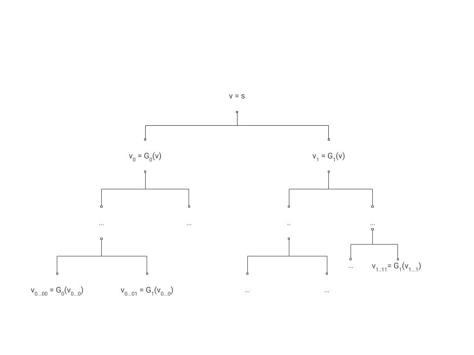
We describe the proof, see also Chapter 6 of Rosulek or Section 8.5 of Katz-Lindell (section 7.5 in 2nd edition) for alternative expositions.
If the PRG Conjecture is true then in particular by the length extension theorem there exists a PRG \(G:\{0,1\}^n\rightarrow\{0,1\}^{2n}\) that maps \(n\) bits into \(2n\) bits. Let’s denote \(G(s)=G_0(s)\circ G_1(s)\) where \(\circ\) denotes concatenation. That is, \(G_0(s)\) denotes the first \(n\) bits and \(G_1(s)\) denotes the last \(n\) bits of \(G(s)\).
For \(i\in\{0,1\}^n\), we define \(f_s(i)\) as
This definition directly corresponds to the depiction in Figure 5.1, where the successive applications of \(G_{b}\) correspond to the recursive labeling procedure.
By the definition above we can see that to evaluate \(f_s(i)\) we need to evaluate the pseudorandom generator \(n\) times on inputs of length \(n\), and so if the pseudorandom generator is efficiently computable then so is the pseudorandom function. Thus, “all” that’s left is to prove that the construction is secure and this is the heart of this proof.
I’ve mentioned before that the first step of writing a proof is convincing yourself that the statement is true, but there is actually an often more important zeroth step which is understanding what the statement actually means. In this case what we need to prove is the following:
We need to show that the security of the PRG \(G\) implies the security of the PRF ensemble \(\{ f_s \}\). Via the contrapositive, this means that we assume that there is an adversary \(A\) that can distinguish in time \(T\) a black box for \(f_s(\cdot)\) from a black-box for a random function with advantage \(\epsilon\). We need to use \(A\) come up with an adversary \(D\) that can distinguish in time \(poly(T)\) an input of the form \(G(s)\) (where \(s\) is random in \(\{0,1\}^n\)) from an input of the form \(y\) where \(y\) is random in \(\{0,1\}^{2n}\) with bias at least \(\epsilon/poly(T)\).
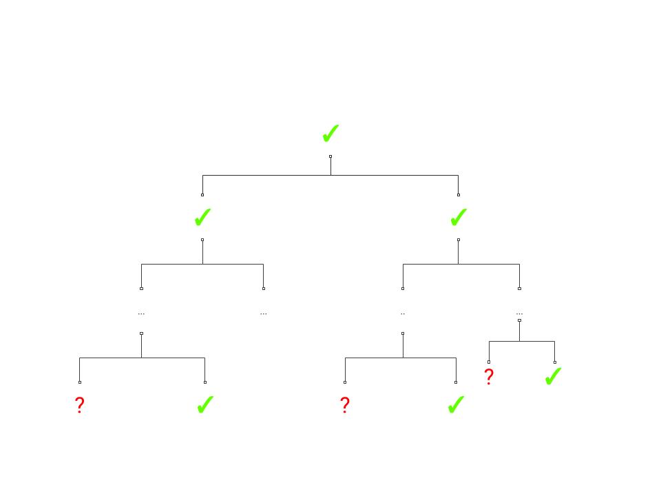
Assume that \(A\) as above is a \(T\)-time adversary that wins in the “PRF game” with advantage \(\epsilon\). Let us consider the “lazy evaluation” implementation of the black box for \(A\) illustrated in Figure 5.2. That is, at every point in time there are nodes in the full binary tree that are labeled and nodes which we haven’t yet labeled. When \(A\) makes a query \(i\), this query corresponds to the path \(i_1\ldots i_n\) in the tree. We look at the lowest (furthest away from the root) node \(v\) on this path which has been labeled by some value \(y\), and then we continue labelling the path from \(v\) downwards until we reach \(i\). In other words, we label the two children of \(v\) by \(G_0(y)\) and \(G_1(y)\), and then if the path \(i\) involves the first child then we label its children by \(G_0(G_0(y))\) and \(G_1(G_0(y))\), and so on and so forth (see Figure 5.3). Note that because \(G_{0}(y)\) and \(G_{1}(y)\) correspond to a single call to \(G\), regardless of whether the traversals continues left or right (i.e. whether the current level corresponds to a value 0 or 1 in \(i\)) we label both children at the same time.
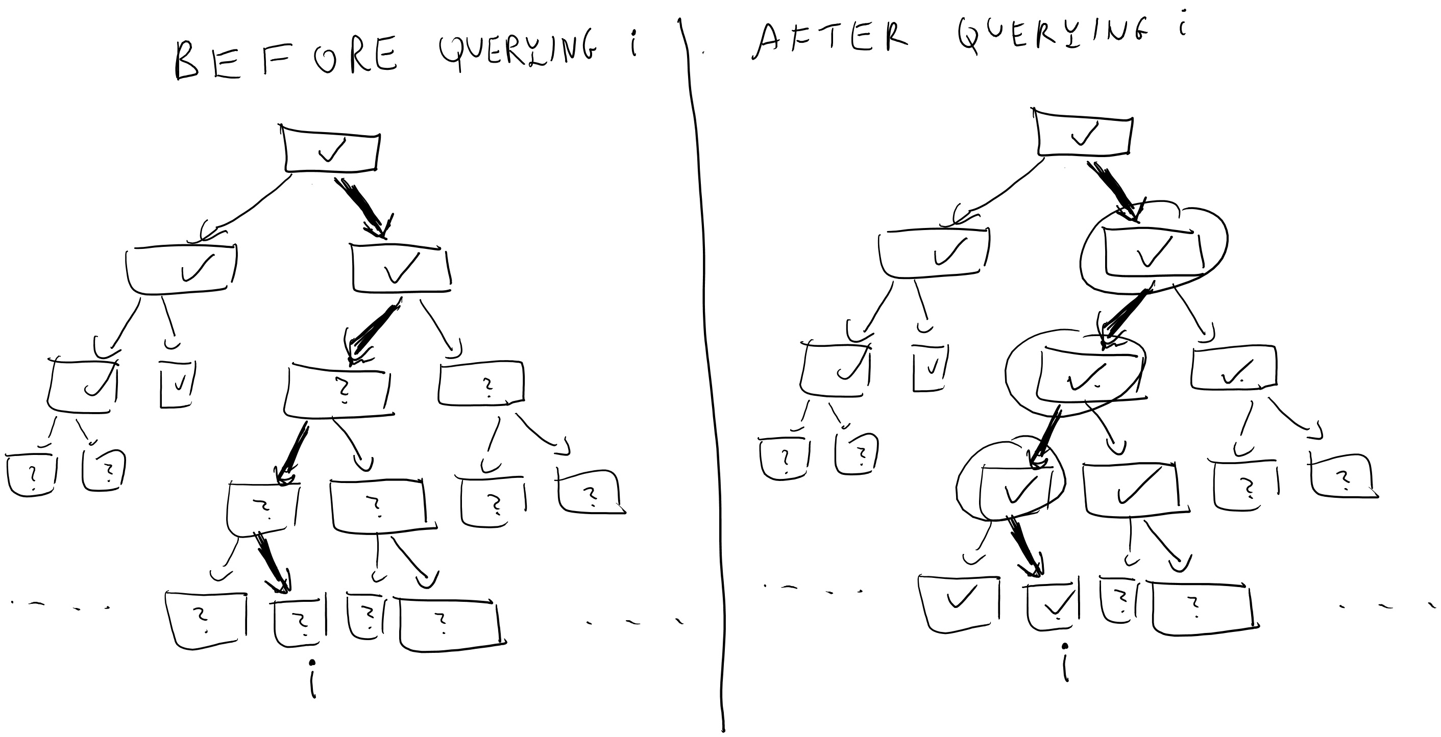
A moment’s thought shows that this is just another (arguably cumbersome) way to describe the oracle that simply computes the map \(i\mapsto f_s(i)\). And so the experiment of running \(A\) with this oracle produces precisely the same result as running \(A\) with access to \(f_s(\cdot)\). Note that since \(A\) has running time at most \(T\), the number of times our oracle will need to label an internal node is at most \(T' \leq 2nT\) (since we label at most \(2n\) nodes for every query \(i\)).
We now define the following \(T'\) hybrids: in the \(j^{th}\) hybrid, we run this experiment but in the first \(j\) times the oracle needs to label internal nodes then it uses independent random labels. That is, for the first \(j\) times we label a node \(v\), instead of letting the label of \(v\) be \(G_b(u)\) (where \(u\) is the parent of \(v\), and \(b\in \{0,1\}\) corresponds to whether \(v\) is the left or right child of \(u\)), we label \(v\) by a random string in \(\{0,1\}^n\).
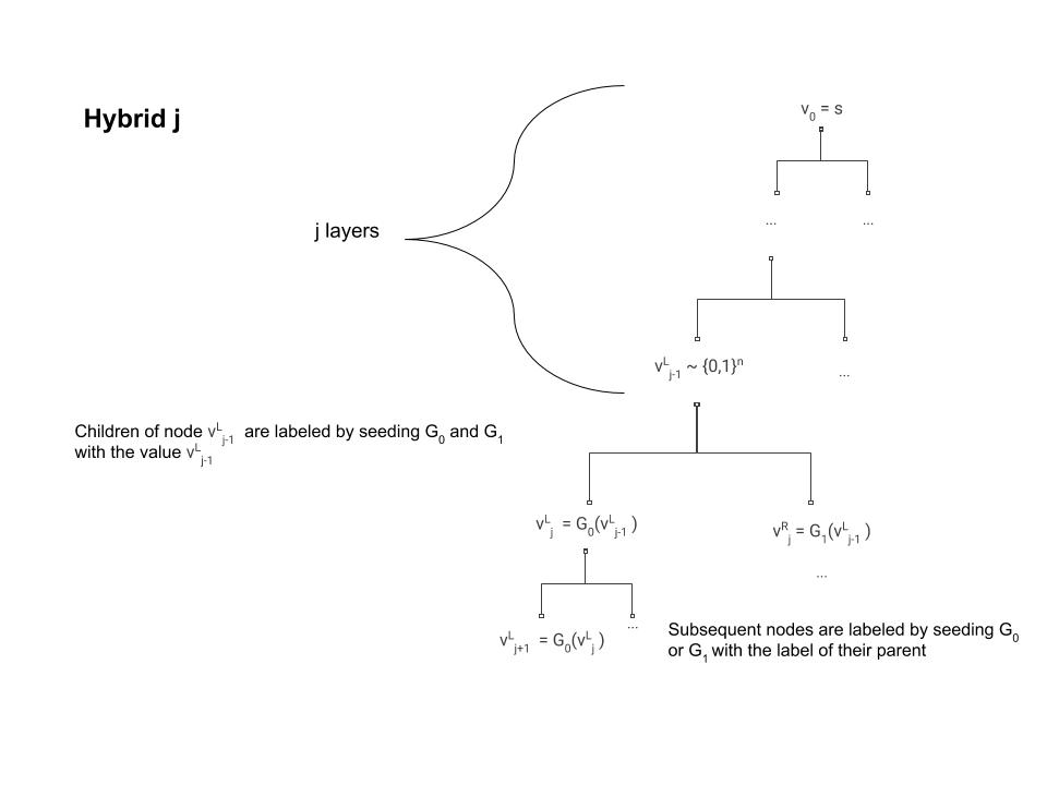
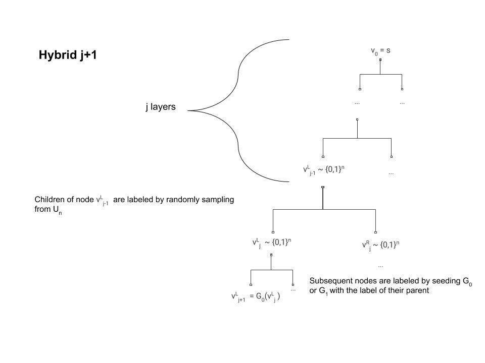
Note that the \(0^{th}\) hybrid corresponds to the case where the oracle implements the function \(i\mapsto f_s(i)\), while in the \(T'^{th}\) hybrid all labels are random and hence implements a random function. By the hybrid argument, if \(A\) can distinguish between the \(0^{th}\) hybrid and the \(T'^{th}\) hybrid with bias \(\epsilon\) then there must exists some \(j\) such that it distinguishes between the \(j^{th}\) hybrid (pictured in Figure 5.4) and the \(j+1^{st}\) hybrid (pictured in Figure 5.5) with bias at least \(\epsilon/T'\). We will use this \(j\) and \(A\) to break the pseudorandom generator.
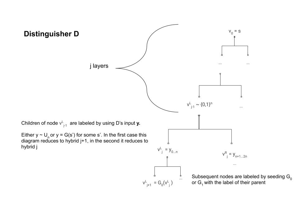
We can now describe our distinguisher \(D\) (see Figure 5.6) for the pseudorandom generator. On input a string \(y\in\{0,1\}^{2n}\) \(D\) will run \(A\) and the \(j^{th}\) oracle inside its belly with one difference- when the time comes to label the \(j^{th}\) node, instead of doing this by applying the pseudorandom generator to the label of its parent \(v\) (which is what should happen in the \(j^{th}\) oracle) it uses its input \(y\) to label the two children of \(v\).
Now, if \(y\) was completely random then we get exactly the distribution of the \(j+1^{st}\) oracle, and hence in this case \(D\) simulates internally the \(j+1^{st}\) hybrid. However, if \(y=G(s)\) for some randomly sampled \(s\in\{0,1\}^n\), though it may not be obvious at first, we actually get the distribution of the \(j^{th}\) oracle.
The equivalence between hybrid \(j\) and distinguisher \(D\) under the condition that \(y=G(s)\) is non obvious, because in hybrid \(j\), the label for the children of \(v_{j-1}^{L}\) was supposed to be the result of applying the pseudorandom generator to the label of \(v_{j-1}^{L}\) and not to some other random string (see Figure 5.6). However, because \(v\) was labeled before the \(j^{th}\) step then we know that it was actually labeled by a random string. Moreover, since we use lazy evaluation we know that step \(j\) is the first time where we actually use the value of the label of \(v\). Hence, if at this point we resampled this label and used a completely independent random string \(s\) then the distribution of \(v_{j-1}^{L}\) and \(s\) would be identical.
The key observations here are:
The output of \(A\) does not directly depend on the internal labels, but only on the labels of the leaves (since those are the only values returned by the oracle).
The label for an internal vertex \(v\) is only used once, and that is for generating the labels for its children.
Hence the distribution of \(y=G(s)\), for \(s\) drawn from \(U_n\), is identical to the distribution, \(G(v_{j-1}^{L})\), of the \(j^{th}\) hybrid, and thus if \(A\) had advantage \(\epsilon\) in breaking the PRF \(\{ f_s \}\) then \(D\) will have advantage \(\epsilon/T'\) in breaking the PRG \(G\) thus obtaining a contradiction.
While this construction reassures us that we can rely on the existence of pseudorandom functions even on days where we remember to take our meds, this is not the construction people use when they need a PRF in practice because it is still somewhat inefficient, making \(n\) calls to the underlying pseudorandom generators. There are constructions (e.g., HMAC) based on hash functions that require stronger assumptions but can use as few as two calls to the underlying function. We will cover these constructions when we talk about hash functions and the random oracle model. One can also obtain practical constructions of PRFs from block ciphers, which we’ll see later in this lecture.
Securely encrypting many messages - chosen plaintext security
Let’s get back to our favorite task of encryption. We seemed to have nailed down the definition of secure encryption, or did we?
Try to think what kind of security guarantees are not provided by the notion of computational secrecy we saw in Definition 2.6
Definition 2.6 talks about encrypting a single message, but this is not how we use encryption in the real world. Typically, Alice and Bob (or Amazon and Boaz) setup a shared key and then engage in many back and forth messages between one another. At first, we might think that this issue of a single long message vs. many short ones is merely a technicality. After all, if Alice wants to send a sequence of messages \((m_1,m_2,\ldots,m_t)\) to Bob, she can simply treat them as a single long message. Moreover, the way that stream ciphers work, Alice can compute the encryption for the first few bits of the message she decides what will be the next bits and so she can send the encryption of \(m_1\) to Bob and later the encryption of \(m_2\). There is some truth to this sentiment, but there are issues with using stream ciphers for multiple messages. For Alice and Bob to encrypt messages in this way, they must maintain a synchronized shared state. If the message \(m_1\) was dropped by the network, then Bob would not be able to decrypt correctly the encryption of \(m_2\).
There is another way in which treating many messages as a single tuple is unsatisfactory. In real life, Eve might be able to have some impact on what messages Alice encrypts. For example, the Katz-Lindell book describes several instances in World War II where Allied forces made particular military maneuver for the sole purpose of causing the Axis forces to send encryptions of messages of the Allies’ choosing. To consider a more modern example, today Google uses encryption for all of its search traffic including (for the most part) the ads that are displayed on the page. But this means that an attacker, by paying Google, can cause it to encrypt arbitrary text of their choosing. This kind of attack, where Eve chooses the message she wants to be encrypted is called a chosen plaintext attack. You might think that we are already covering this with our current definition that requires security for every pair of messages and so in particular this pair could be chosen by Eve. However, in the case of multiple messages, we would want to allow Eve to be able to choose \(m_2\) after she saw the encryption of \(m_1\).
All that leads us to the following definition, which is a strengthening of our definition of computational security:
An encryption scheme \((E,D)\) is secure against chosen plaintext attack (CPA secure) if for every polynomial time \(Eve\), Eve wins with probability at most \(1/2+negl(n)\) in the game defined below:
- The key \(k\) is chosen at random in \(\{0,1\}^n\) and fixed.
- Eve gets the length of the key \(1^n\) as input.1
- Eve interacts with \(E\) for \(t=poly(n)\) rounds as follows: in the \(i^{th}\) round, Eve chooses a message \(m_i\) and obtains \(c_i= E_k(m_i)\).
- Then Eve chooses two messages \(m_0,m_1\), and gets \(c^* = E_k(m_b)\) for \(b\leftarrow_R\{0,1\}\).
- Eve continues to interact with \(E\) for another \(poly(n)\) rounds, as in Step 3.
- Eve wins if she outputs \(b\).
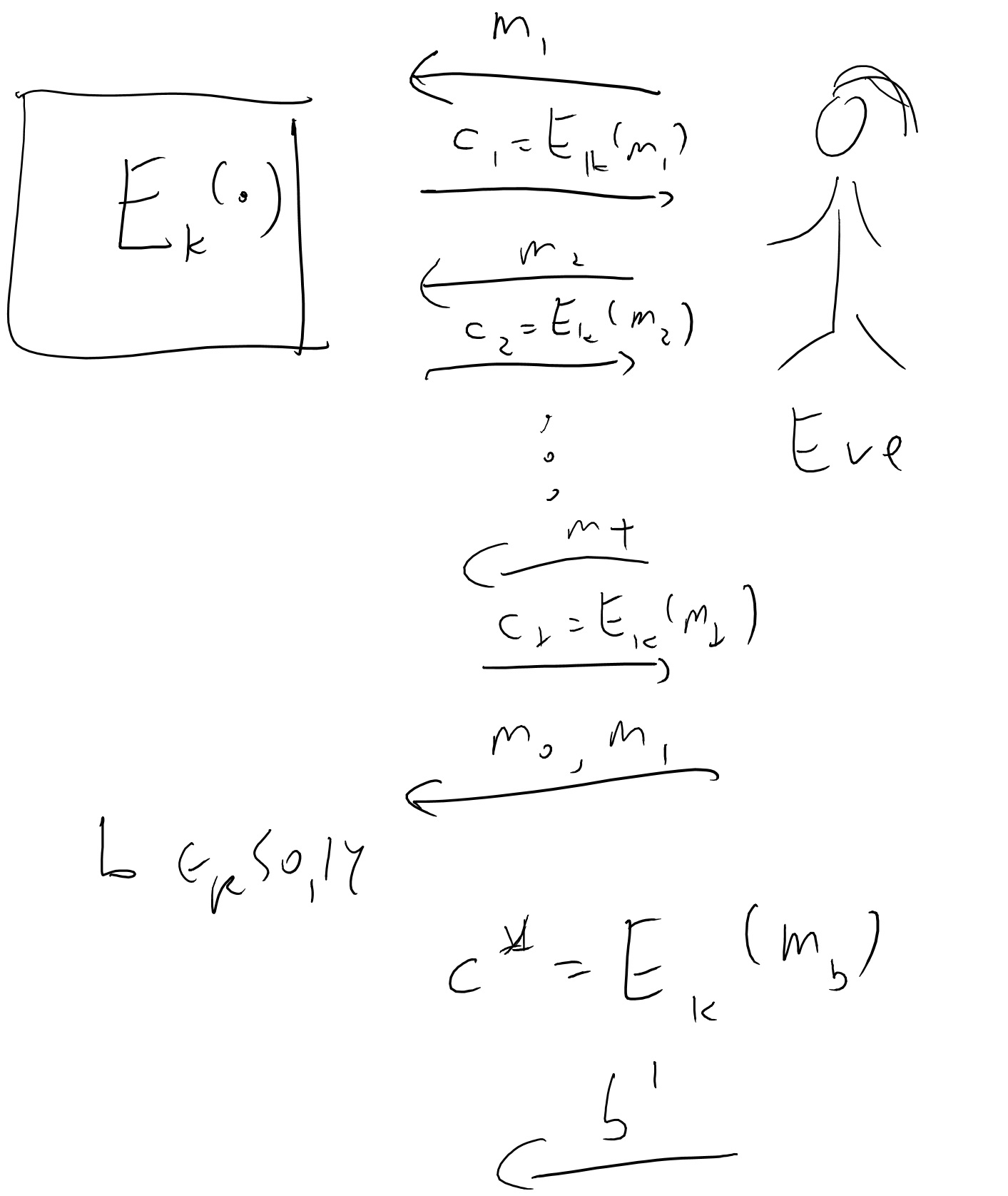
Definition 5.3 is illustrated in Figure 5.7. Our previous notion of computational secrecy (i.e., Definition 2.6) corresponds to the case that we skip Steps 3 and 5 above. Since Steps 3 and 5 only give the adversary more power (and hence is only more likely to win), CPA security (Definition 5.3) is stronger than computational secrecy (Definition 2.6), in the sense that every CPA secure encryption \((E,D)\) is also computationally secure. It turns out that CPA security is strictly stronger, in the sense that without modification, our stream ciphers cannot be CPA secure. In fact, we have a stronger, and intially somewhat surprising theorem:
There is no CPA secure \((E,D)\) where \(E\) is deterministic.
The proof is very simple: Eve will only use a single round of interacting with \(E\) where she will ask for the encryption \(c_1\) of \(0^\ell\). In the second round, Eve will choose \(m_0=0^{\ell}\) and \(m_1=1^{\ell}\), and get \(c^*=E_k(m_b)\) she will then output \(0\) if and only if \(c^*=c_1\).
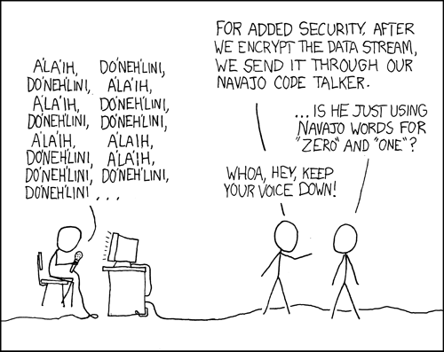
This proof is so simple that you might think it shows a problem with the definition, but it is actually a real problem with security. If you encrypt many messages and some of them repeat themselves, it is possible to get significant information by seeing the repetition pattern (cue the XKCD cartoon again, see Figure 5.8). To avoid this issue we need to use a randomized (or probabilistic) encryption, such that if we encrypt the same message twice we won’t see two copies of the same ciphertext.2 But how do we do that? Here pseudorandom functions come to the rescue:
Suppose that \(\{ f_s \}\) is a PRF collection where \(f_s:\{0,1\}^n\rightarrow\{0,1\}^\ell\), then the following is a CPA secure encryption scheme: \(E_s(m)=(r,f_s(r)\oplus m)\) where \(r \leftarrow_R \{0,1\}^n\), and \(D_s(r,z)=f_s(r)\oplus z\).
I leave to you to verify that \(D_s(E_s(m))=m\). We need to show the CPA security property. As is usual in PRF-based constructions, we first show that this scheme will be secure if \(f_s\) was an actually random function, and then use that to derive security.
Consider the game above when played with a completely random function and let \(r_i\) be the random string chosen by \(E\) in the \(i^{th}\) round and \(r^*\) the string chosen in the last round. We start with the following simple but crucial claim:
Claim: The probability that \(r^*=r_i\) for some \(i\) is at most \(T/2^n\).
Proof of claim: For any particular \(i\), since \(r^*\) is chosen independently of \(r_i\), the probability that \(r^*=r_i\) is \(2^{-n}\). Hence the claim follows from the union bound. QED
Given this claim we know that with probability \(1-T/2^n\) (which is \(1-negl(n)\)), the string \(r^*\) is distinct from any string that was chosen before. This means that by the lazy evaluation principle, if \(f_s(\cdot)\) is a completely random function then the value \(f_s(r^*)\) can be thought of as being chosen at random in the final round independently of anything that happened before. But then \(f_s(r^*)\oplus m_b\) amounts to simply using the one-time pad to encrypt \(m_b\). That is, the distributions \(f_s(r^*)\oplus m_0\) and \(f_s(r^*)\oplus m_1\) (where we think of \(r^*,m_0,m_1\) as fixed and the randomness comes from the choice of the random function \(f_s(\cdot)\)) are both equal to the uniform distribution \(U_n\) over \(\{0,1\}^n\) and hence Eve gets absolutely no information about \(b\).
This shows that if \(f_s(\cdot)\) was a random function then Eve would win the game with probability at most \(1/2\). Now if we have some efficient Eve that wins the game with probability at least \(1/2+\epsilon\) then we can build an adversary \(A\) for the PRF that will run this entire game with black box access to \(f_s(\cdot)\) and will output \(1\) if and only if Eve wins. By the argument above, there would be a difference of at least \(\epsilon\) in the probability it outputs \(1\) when \(f_s(\cdot)\) is random vs when it is pseudorandom, hence contradicting the security property of the PRF.
Pseudorandom permutations / block ciphers
Now that we have pseudorandom functions, we might get greedy and want such functions with even more magical properties. This is where the notion of pseudorandom permutations comes in.
::: {.definition title=“Pseudorandom permutations” #PRPdef} Let \(\ell:\N \rightarrow \N\) be some function that is polynomially bounded (i.e., there are some \(0<c<C\) such that \(n^c < \ell(n) < n^C\) for every \(n\)). A collection of functions \(\{ f_s \}\) where \(f_s:\{0,1\}^{\ell} \rightarrow\{0,1\}^{\ell}\) for \(\ell=\ell(|s|)\) is called a pseudorandom permutation (PRP) collection if:
- It is a pseudorandom function collection (i.e., the map \(s,x \mapsto f_s(x)\) is efficiently computable and there is no efficient distinguisher between \(f_s(\cdot)\) with a random \(s\) and a random function).
- Every function \(f_s\) is a permutation of \(\{0,1\}^\ell\) (i.e., a one to one and onto map).
- There is an efficient algorithm that on input \(s,y\) returns \(f_s^{-1}(y)\). The parameter \(n\) is known as the key length of the pseudorandom permutation collection and the parameter \(\ell=\ell(n)\) is known as the input length or block length. Often, \(\ell=n\) and so in most cases you can safely ignore this distinction.
At first look ?? ?? might seem not to make sense, since on one hand it requires the map \(x \mapsto f_s(x)\) to be a permutation, but on the other hand it can be shown that with high probability a random map \(H:\{0,1\}^\ell \rightarrow \{0,1\}^\ell\) will not be a permutation. How can then such a collection be pseudorandom? The key insight is that while a random map might not be a permutation, it is not possible to distinguish with a polynomial number of queries between a black box that computes a random function and a black box that computes a random permutation. Understanding why this is the case, and why this means that ?? ?? is reasonable, is crucial to getting intuition to this notion, and so I suggest you pause now and make sure you understand these points.
As usual with a new concept, we want to know whether it is possible to achieve it and whether it is useful. The former is established by the following theorem:
If the PRF conjecture holds (and hence by Theorem 5.1 also if the PRG conjecture holds) then there exists a pseudorandom permutation collection.
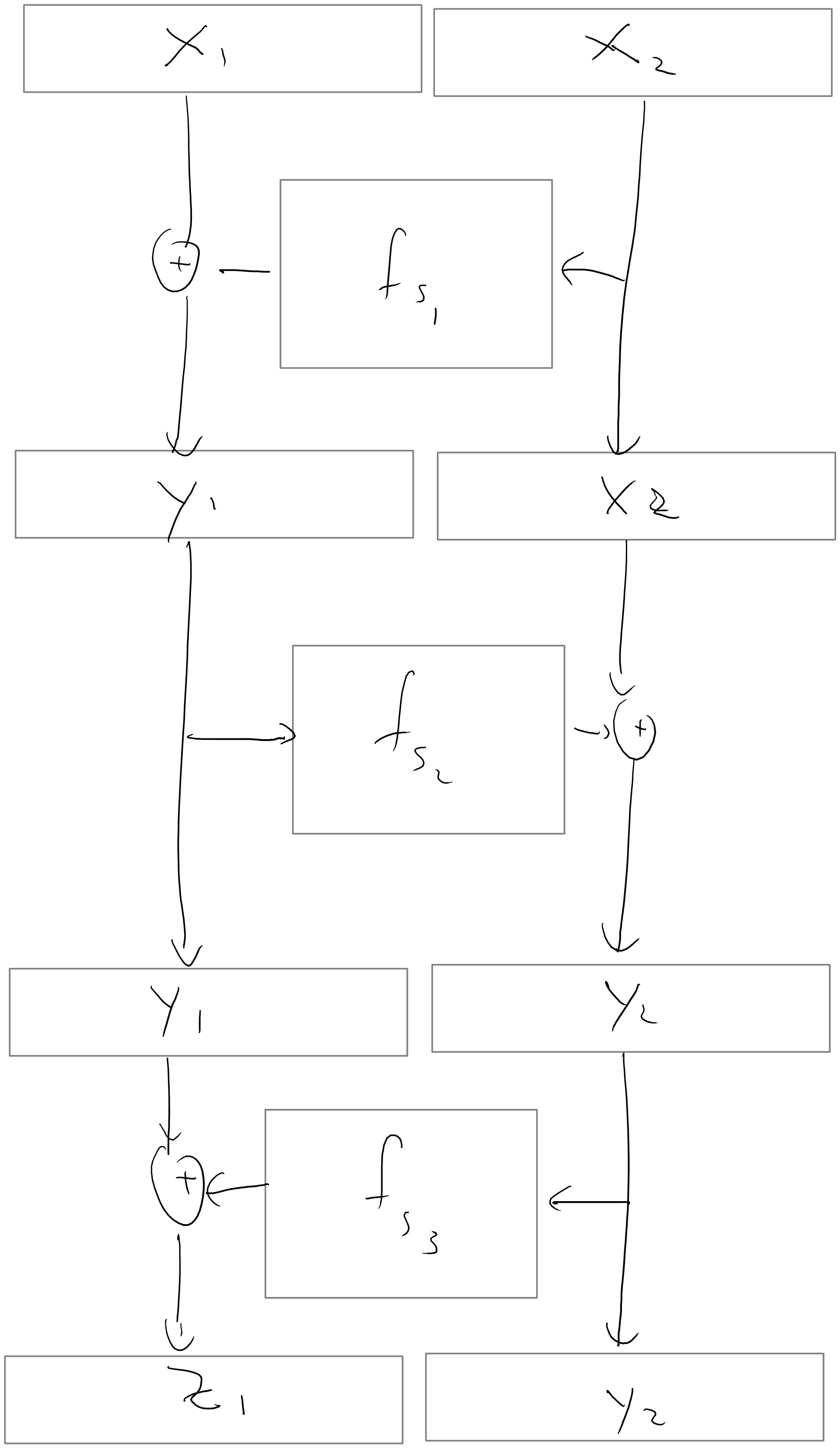
Figure 5.9 illustrates the construction of a pseudorandom permutation from a pseudorandom function. The construction (known as the Luby-Rackoff construction) uses several rounds of what is known as the Feistel Transformation that maps a function \(f:\{0,1\}^n \rightarrow \{0,1\}^n\) into a permutation \(g:\{0,1\}^{2n} \rightarrow \{0,1\}^{2n}\) using the map \((x,y) \mapsto (x,f(x) \oplus y)\).
Specifically, given a PRF family \(\{f_s\}\) with \(n\)-bit keys, inputs, and outputs, our candidate PRP family will be called \(\{p_{s_1,s_2,s_3}\}\). Here, \(p_{s_1,s_2, s_3}:\{0,1\}^{2n} \to \{0,1\}^{2n}\) is calculated on input \((x_1, x_2) \in \{0,1\}^{2n}\) as follows (see Figure 5.9):
- First, map \((x_1, x_2) \mapsto (y_1, x_2)\), where \(y_1 = x_1 \oplus f_{s_1}(x_2)\).
- Next, map \((y_1, x_2) \mapsto (y_1, y_2)\), where \(y_2 = x_2 \oplus f_{s_2}(y_1)\).
- Next, map \((y_1, y_2) \mapsto (z_1, y_2)\), where \(z_1 = y_1 \oplus f_{s_3}(y_2)\).
- Finally, output \(p_{s_1,s_2,s_3}(x_1,x_2) = (z_1, y_2)\).
Each of the first three steps above corresponds to a single round of the Feistel transformation, which is easily seen to be both efficiently computable and efficiently invertible. In fact, we can efficiently calculate \(p_{s_1,s_2,s_3}^{-1}(z_1, y_2)\) for an arbitrary string \((z_1,y_2) \in \{0,1\}^{2n}\) by running the above three rounds of Feistel transformations in reverse order.
Thus, the real challenge in proving Theorem 5.6 is not showing that \(\{p_{s_1,s_2,s_3}\}\) is a valid permutation, but rather showing that it is pseudorandom. The details of remainder of this proof are a bit technical, and can be safely skipped on a first reading.
Intuitively, the argument goes like this. Consider an oracle \(\mathcal{O}\) for \(p_{s_1,s_2,s_3}\) that answers an adversary’s query \((x_1, x_2)\) by carrying out the three Feistel transformations outlined above and outputting \((z_1, y_2)\). First, we’ll show that with high probability, \(\mathcal{O}\) will never encounter the same intermediate string \(y_1\) twice, over the course of all queries (unless the adversary makes a duplicate query). Since the string \(y_1\), calculated in Step 1, determines the input on which \(f_{s_2}\) is evaluated in Step 2, it follows that the strings \(y_2\) calculated in Step 2 will appear to be chosen independently and at random. In particular, they too will be pairwise distinct with high probability. Since the string \(y_2\) is in turn passed as input to \(f_{s_3}\) in Step 3, it follows that the strings \(z_1\) encountered over the course of all queries will also appear to be chosen independently and at random. Ultimately, this means that the oracle’s outputs \((z_1, y_2)\) will look like freshly independent, random strings.
To make this reasoning precise, notice first that it suffices to establish the security of a variant of \(p_{s_1,s_2,s_3}\) in which the pseudorandom functions \(f_{s_1}\), \(f_{s_2}\), and \(f_{s_3}\) used in the construction are replaced by truly random functions \(h_1,h_2,h_3 : \{0,1\}^n \to \{0,1\}^n\). Call this variant \(p_{h_1,h_2,h_3}\). Indeed, the assumption that \(\{f_s\}\) is a PRF collection tells us that making this change has only a negligible effect on the output of an adversary with oracle access to \(p\). With this in mind, our job is to show that for every efficient adversary \(A\), the difference \(|\Pr[A^{p_{h_1,h_2,h_3}(\cdot)}(1^n)=1] - \Pr[A^{H(\cdot)}(1^n)=1]|\) is negligible. In this expression, the first probability is taken over the choice of the random functions \(h_1,h_2,h_3 :\{0,1\}^n \to \{0,1\}^n\) used in the Feistel transformation, and the second probability is taken over the random function \(H : \{0,1\}^{2n} \to \{0,1\}^{2n}\). To simplify matters, suppose without loss of generality that \(A\) always makes \(q(n)\) distinct queries to its oracle, denoted \((x_1^{(1)}, x_2^{(1)}), \ldots, (x_1^{(q(n))}, x_2^{(q(n))})\) in order. Similarly, let \(y_1^{(i)}, y_2^{(i)}, z_1^{(i)}\) denote the intermediate strings calculated in the three rounds of the Feistel transformation. Here, \(q\) is a polynomial in \(n\).
Consider the case in which the adversary \(A\) is interacting with the oracle for \(p_{h_1,h_2,h_3}\), as opposed to the random oracle. Let us say that a collision occurs at \(y_1\) if for some \(1 \le i < j \le q(n)\), the string \(y_1^{(i)}\) computed while answering \(A\)’s \(i\)th query coincides with the string \(y_1^{(j)}\) computed while answering \(A\)’s \(j\)th query. We claim the probability that a collision occurs at \(y_1\) is negligibly small. Indeed, if a collision occurs at \(y_1\), then \(y_1^{(i)} = y_1^{(j)}\) for some \(i \neq j\). By the construction of \(p_{h_1,h_2,h_3}\), this means that \(x_1^{(i)} \oplus h_1(x_2^{(i)}) = x_1^{(j)} \oplus h_1(x_2^{(j)})\). In particular, it cannot be the case that \(x_1^{(i)} \neq x_1^{(j)}\) and \(x_2^{(i)} = x_2^{(j)}\). Since we assumed that \(A\) makes distinct queries to its oracle, it follows that \(x_2^{(i)} \neq x_2^{(j)}\) and hence that \(h_1(x_2^{(i)})\) and \(h_1(x_2^{(j)})\) are uniform and independent. In other words, \(\Pr[y_1^{(i)} = y_1^{(j)}] = \Pr[x_1^{(i)} \oplus f_1(x_2^{(i)}) = x_1^{(j)} \oplus f_1(x_2^{(j)})] = 2^{-n}\). Taking a union bound over all choices of \(i\) and \(j\), we see that the probability of a collision at \(y_1\) is at most \(q(n)^2/2^n\), which is negligible.
Next, define a collision at \(y_2\), by a pair of queries \(1 \le i < j \le q(n)\) such that \(y_2^{(i)} = y_2^{(j)}\). We argue that the probability of a collision at \(y_2\) is also negligible, provided that we condition on the overwhelmingly likely event that no collision occurs at \(y_1\). Indeed, if \(y_1^{(i)} \neq y_1^{(j)}\) for all \(i \neq j\), then \(h_2(y_1^{(1)}), \ldots, h_2(y_1^{(q(n))})\) are distribued independently and uniformly at random. In particular, we have \(\Pr[y_2^{(i)} = y_2^{(j)} \mid \text{no collision at }y_1] = 2^{-n}\), which is negligible even after taking a union bound over all \(i\) and \(j\). The same argument applied to the third round of the Feistel transformation similarly shows that, conditioned on the overwhelmingly likely event that no collision occurs at \(y_1\) or \(y_2\), the strings \(z_1^{(1)}, \ldots, z_1^{(i)}\) for \(1 \le i \le q(n)\) are also distributed as fresh, independent, random strings. At this point, we’ve shown that the adversary cannot distinguish the outputs \((z_1^{(1)}, y_2^{(1)}), \ldots, (z_1^{(q(n))}, y_2^{(q(n))})\) of the oracle for \(p_{h_1,h_2,h_3}\) from the outputs of a random oracle unless an event with negligibly small probability occurs. We conclude that the collection \(\{p_{h_1,h_2,h_3}\}\), and hence our original collection \(\{p_{s_1,s_2,s_3}\}\), is a secure PRP collection.
For more details regarding this proof, see Section 4.5 in Boneh Shoup or Section 8.6 (7.6 in 2nd ed) in Katz-Lindell, whose proof was used as a model for ours.
The construction in the proof of Theorem 5.6 constructed a PRP \(p\) by performing \(3\) rounds of the Feistel transformation with a known PRF \(f\). It is an interesting exercise to try to show that doing just \(1\) or \(2\) rounds of the Feistel transformation does not suffice to achieve a PRP. Hint: consider an adversary that makes queries of the form \((x_1, x_2)\) where \(x_2\) is held fixed and \(x_1\) is varied.
The more common name for a pseudorandom permutation is block cipher (though typically block ciphers are expected to meet additional security properties on top of being PRPs). The constructions for block ciphers used in practice don’t follow the construction of Theorem 5.6 (though they use some of the ideas) but have a more ad-hoc nature.
One of the first modern block ciphers was the Data Encryption Standard (DES) constructed by IBM in the 1970’s. It is a fairly good cipher- to this day, as far as we know, it provides a pretty good number of security bits compared to its key length. The trouble is that its key is only \(56\) bits long, which is no longer outside the reach of modern computing power. (It turns out that subtle variants of DES are far less secure and fall prey to a technique known as differential cryptanalysis; the IBM designers of DES were aware of this technique but kept it secret at the behest of the NSA.)
Between 1997 and 2001, the U.S. National Institute of Standards and Technology (NIST) ran a competition to replace DES which resulted in the adoption of the block cipher Rijndael as the new advanced encryption standard (AES). It has a block size (i.e., input length) of 128 bits and a key size (i.e., seed length) of 128, 196, or 256 bits.
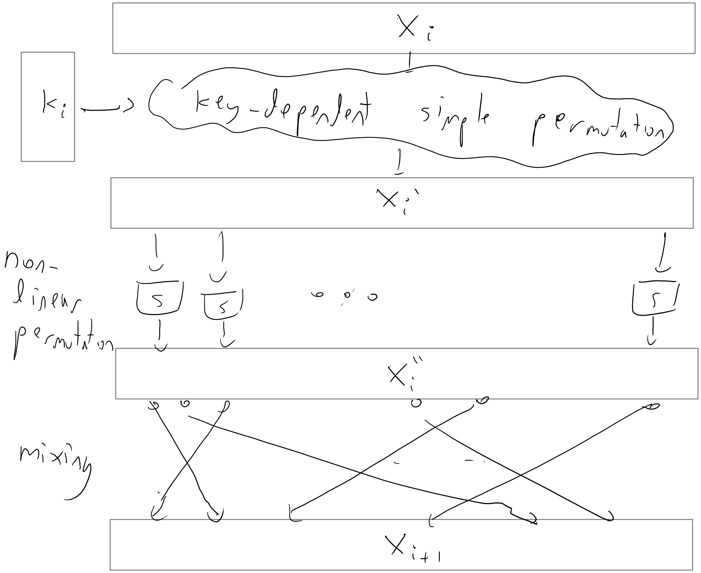
The actual construction of AES (or DES for that matter) is not extremely illuminating, but let us say a few words about the general principle behind many block ciphers. They are typically constructed by repeating one after the other a number of very simple permutations (see Figure 5.10). Each such iteration is called a round. If there are \(t\) rounds, then the key \(k\) is typically expanded into a longer string, which we think of as a \(t\) tuple of strings \((k_1,\ldots,k_t)\) via some pseudorandom generator known as the key scheduling algorithm. The \(i\)-th string in the tuple is known as the round key and is used in the \(i^{th}\) round. Each round is typically composed of several components: there is a “key mixing component” that performs some simple permutation based on the key (often as simply as XOR’ing the key), there is a “mixing component” that mixes the bits of the block so that bits that were initially nearby don’t stay close to one another, and then there is some non-linear component (often obtained by applying some simple non-linear functions known as “S boxes” to each small block of the input) that ensures that the overall cipher will not be an affine function. Each one of these operations is an easily reversible operations, and hence decrypting the cipher simply involves running the rounds backwards.
Encryption modes
How do we use a block cipher to actually encrypt traffic? Well we could use it as a PRF in the construction above, but in practice people use other ways.3
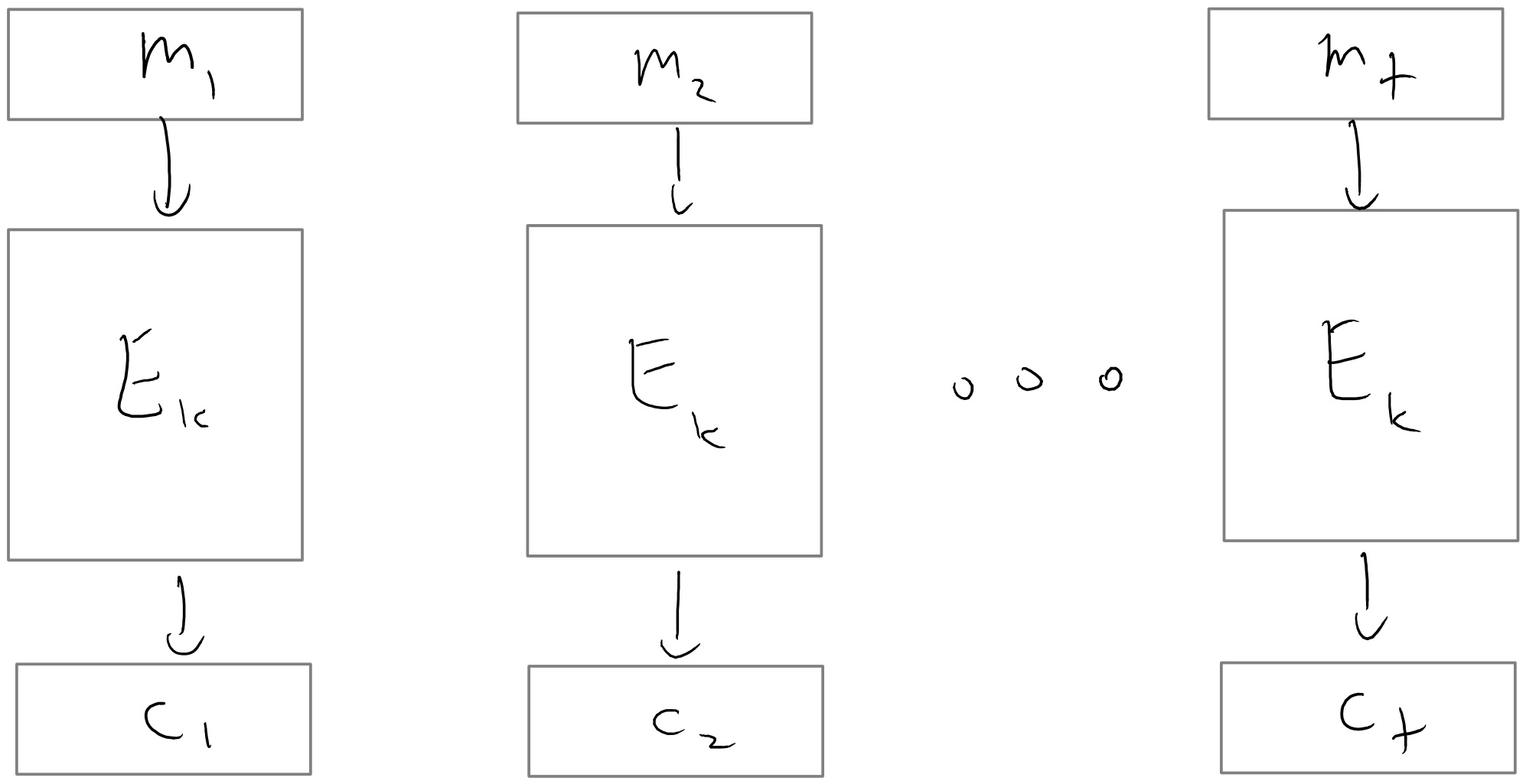
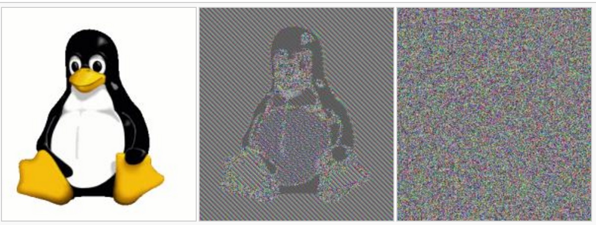
The most natural approach would be that to encrypt a message \(m\), we simply use \(p_s(m)\) where \(\{ p_s \}\) is the PRP/block cipher. This is known as the electronic code book (ECB) mode of a block cipher (see Figure 5.11). Note that we can easily decrypt since we can compute \(p_s^{-1}(m)\). If the PRP \(\{p_s\}\) only accepts inputs of a fixed length \(\ell\), we can use ECB mode to encrypt a message \(m\) whose length is a multiple of \(\ell\) by writing \(m = (m_1, m_2, \ldots, m_t)\), where each block \(m_i\) has length \(\ell\), and then encrypting each block \(m_i\) separately. The ciphertext output by this encryption scheme is \((p_s(m_1), \ldots, p_s(m_t))\). A major drawback of ECB mode is that it is a deterministic encryption scheme and hence cannot be CPA secure. Moreover, this is actually a real problem of security on realistic inputs (see Figure 5.12), so ECB mode should never be used.
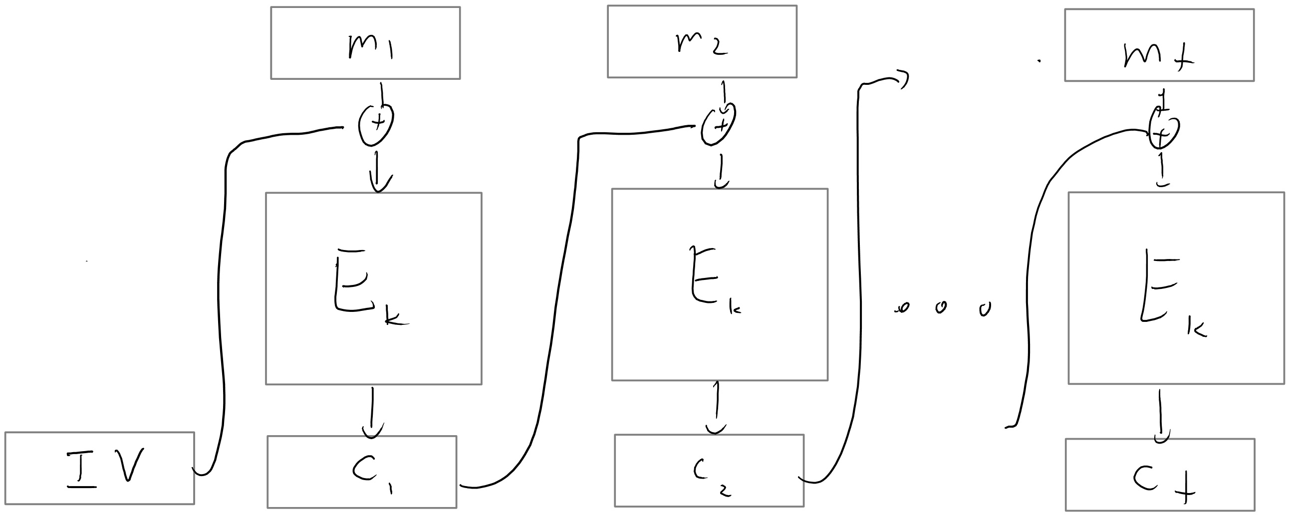
A more secure way to use a block cipher to encrypt is the cipher block chaining (CBC) mode. The idea of cipher block chaining is to encrypt the blocks of a message \(m = (m_1, \ldots, m_t)\) sequentially. To encrypt the first block \(m_1\), we XOR \(m_1\) with a random string known as the initialization vector, or \(\ensuremath{\mathit{IV}}\), before applying the block cipher \(p_s\). To encrypt one of the later blocks \(m_i\), where \(i > 1\), we XOR \(m_i\) with the encryption of \(m_{i-1}\) before applying the block cipher \(p_s\). Formally, the ciphertext consists of the tuple \((\ensuremath{\mathit{IV}}, c_1, \ldots, c_t)\), where \(\ensuremath{\mathit{IV}}\) is chosen uniformly at random and \(c_i = p_s(c_{i-1} \oplus m_i)\) for \(1 \le i \le t\) (we use the convention that \(c_0 = \ensuremath{\mathit{IV}}\)). This encryption process is depicted in Figure 5.13. In order to decrypt \((\ensuremath{\mathit{IV}}, c_1, \ldots, c_t)\), we simply calculate \(m_i = p_s^{-1}(c_i) \oplus c_{i-1}\) for \(1 \le i \le t\). Note that if we lose the block \(c_i\) to traffic in the CBC mode, then we are unable to decrypt the next block \(c_{i+1}\), but we can recover from that point onwards.
On the one hand, CBC mode is vastly superior to a simple electronic codebook since CBC mode with a random \(\ensuremath{\mathit{IV}}\) is CPA secure (proving this is an excellent exercise). On the other hand, CBC mode suffers from the drawback that the encryption process cannot be parallelized: the ciphertext block \(c_i\) must be computed before \(c_{i+1}\).
In the output feedback (OFB) mode we first encrypt the all zero string using CBC mode to get a sequence \((y_1,y_2,\ldots)\) of pseudorandom outputs that we can use as a stream cipher. To transmit a message \(m \in \{0,1\}^*\), we send the XOR of \(m\) with the bits output by this stream cipher, along with the \(\ensuremath{\mathit{IV}}\) used to generate the sequence. The receiver can decrypt a ciphertext \((\ensuremath{\mathit{IV}}, c)\) by first using \(\ensuremath{\mathit{IV}}\) to recover \((y_1, y_2, \ldots)\), and then taking the XOR of \(c\) with the appropriate number of bits from this sequence. Like CBC mode, OFB mode is CPA secure when \(\ensuremath{\mathit{IV}}\) is chosen at random. Some advantages of OFB mode over CBC mode include the ability for the sender to precompute the sequence \((y_1, y_2, \ldots)\) well before the message to be encrypted is known, as well as the fact that the underlying function \(p_s\) used to generate \((y_1, y_2, \ldots)\) only needs to be a PRF (not necessarily a PRP).
Perhaps the simplest mode of operation is counter (CTR) mode where we convert a block cipher to a stream cipher by using the stream \(p_s(\ensuremath{\mathit{IV}}),p_s(\ensuremath{\mathit{IV}}+1),p_s(\ensuremath{\mathit{IV}}+2),\ldots\) where \(\ensuremath{\mathit{IV}}\) is a random string in \(\{0,1\}^n\) which we identify with \([2^n]\) (and perform addition modulo \(2^n\)). That is, to encrypt a message \(m = (m_1, \ldots, m_t)\), we choose \(\ensuremath{\mathit{IV}}\) at random, and output \((\ensuremath{\mathit{IV}}, c_1, \ldots, c_t)\), where \(c_i = p_s(\ensuremath{\mathit{IV}} + i) \oplus m_i\) for \(1 \le i \le t\). Decryption is performed similarly. For a modern block cipher, CTR mode is no less secure than CBC or OFB, and in fact offers several advantages. For example, CTR mode can easily encrypt and decrypt blocks in parallel, unlike CBC mode. In addition, CTR mode only needs to evaluate \(p_s\) once to decrypt any single block of the ciphertext, unlike OFB mode.
A fairly comprehensive study of the different modes of block ciphers is in this document by Rogaway. His conclusion is that if we simply consider CPA security (as opposed to the stronger notions of chosen ciphertext security we’ll see in the next lecture) then counter mode is the best choice, but CBC, OFB and CFB are widely implemented due to legacy reasons. ECB should not be used (except as a building block as part of a construction achieving stronger security).
Optional, Aside: Broadcast Encryption
At the beginning of this chapter, we saw the proof of Theorem 5.1, which states that the PRG Conjecture implies the existence of a secure PRF collection. At the heart of this proof was a rather clever construction based on a binary tree. As it turns out, similar tree constructions have been used time and again to solve many other problems in cryptography. In this section, we will discuss just one such application of these tree constructions, namely broadcast encryption.
Let’s put ourselves in the shoes of Hollywood executives facing the following problem: we’ve just released a new movie for sale (in the form of a download or a Blu-ray disc), and we’d like to prevent it from being pirated. On the one hand, consumers who’ve purchased a copy of the movie should be able to watch it on certain approved, standalone devices such as TVs and Blu-ray players without needing an external internet connection. On the other hand, to minimize the risk of piracy, these consumers should not have access to the movie data itself.
One way to protect the movie data, which we model as a string \(x\), is to provide consumers with a secure encryption \(E_k(x)\) of the data. Although the secret key \(k\) used to encrypt the data is hidden from consumers, it is provided to device manufacturers so that they can embed it in their TVs and Blu-ray players in some secure, tamper-resistant manner. As long as the key \(k\) is never leaked to the public, this system ensures that only approved devices can decrypt and play a consumer’s copy of the movie. For this reason, we will sometimes refer to \(k\) as the device key. This setup is depicted in Figure 5.14.

Unfortunately, if we were to implement this scheme exactly as written, it would almost certainly be broken in a matter of days. After all, as soon as even a single device is hacked, the device key \(k\) would be revealed. This would allow the public to access our movie’s data, as well as the data for all future movies we release for these devices! This latter consequence is one that we would certainly want to avoid, and doing so requires the notion of distinct, revocable keys:
For our purposes, a broadcast encryption scheme consists of:
A set of \(m\) distinct devices (or device manufacturers), each of which has access to one of the \(n\)-bit device keys \(k_1, \ldots, k_m\).
A decryption algorithm \(D\) that receives as input a ciphertext \(y\) and a key \(k_i\).
An encryption algorithm \(E\) that receives as input a plaintext \(x\), a key \(k_{master}\), and a revocation set \(R \subseteq [m]\) of devices (or device manufacturers) that are no longer to be trusted.
Intuitively, a broadcast encryption scheme is secure if \(D_{k_i}\) can successfully recover \(x\) from \(E_{k_{master}, R}(x)\) whenever \(i \notin R\), but fails to do so whenever \(i \in R\). In our example of movie piracy, such an encryption scheme would allow us to revoke certain device keys \(k_i\) when we find out that they have been leaked. To revoke a key \(k_i\), we would simply include \(i \in R\) when encrypting all future movies. Doing so prevents \(k_i\) from being used to decrypt these movies. Crucially, revoking the key \(k_i\) of the hacked device \(i\) doesn’t prevent a secure device \(j \neq i\) from continuing to perform decryption on future movie releases; this is exactly what we want in our system.
For the sake of brevity, we will not provide a formal definition of security for broadcast encryption schemes, although this can and has been done. Instead, in the remainder of this section, we will describe a couple examples of broadcast encryption schemes, one of which makes clever use of a tree construction, as promised.
The simplest construction of a broadcast encryption scheme involves letting \(k_{master} = (k_1, \ldots, k_m)\) be the collection of all device keys and letting \(E_{k_{master}, R}(x)\) be the concatenation over all \(i \notin R\) of a secure encryption \(E_{k_i}(x)\). Device \(i\) performs decryption by looking up the relevant substring \(E_{k_i}(x)\) of the ciphertext and decrypting it with \(k_i\). Intuitively, with this scheme, if \(x\) represents our movie data and there are \(m \approx\) one million devices, then \(E_{k_{master}, R}(x)\) is just an encryption of one million copies of the movie (one for each device key). Revoking the key \(k_i\) amounts to only encrypting \(999,999\) copies of all future movies, so that device \(i\) can no longer perform decryption.
Clearly, this simple solution to the broadcast encryption problem has two serious inefficiencies: the length of the master key is \(O(nm)\), and the length of each encryption is \(O(|x|m)\). One way to address the former problem is to use a key derivation function. That is, we can shorten the master key by choosing a fixed PRF collection \(\{f_k\}\), and calculating each device key \(k_i\) by the rule \(k_i = f_{k_{master}}(i)\). The latter problem can be addressed using a technique known as hybrid encryption. In hybrid encryption, we encrypt \(x\) by first choosing an ephemeral key \(\hat k \leftarrow_R \{0,1\}^n\), encrypting \(\hat k\) using each device key \(k_i\) where \(i \notin R\), and then outputting the concatenation of these strings \(E_{k_i}(\hat k)\), along with a single encryption \(E_{\hat k}(x)\) of the movie using the ephermal key. Incorporating these two optimizations reduces the length of \(k_{master}\) to \(O(n)\) and the length of each encryption to \(O(nm + |x|)\).
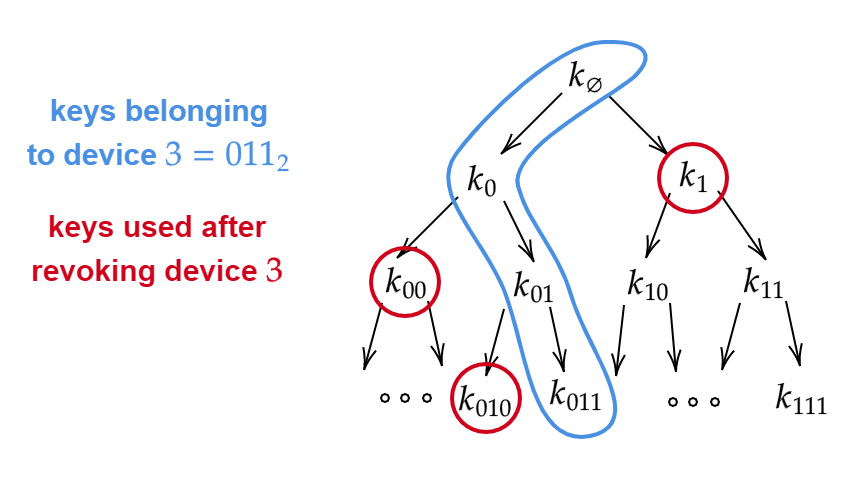
It turns out that we can construct a broadcast encryption scheme with even shorter ciphertexts by considering a tree of keys (see Figure 5.15). The root of this tree is labeled \(k_{\varnothing}\), its children are \(k_0\) and \(k_1\), their children are \(k_{00}, k_{01}, k_{10}, k_{11}\), and so on. The depth of the tree is \(\log_2 m\), and the value of each key in the tree is decided uniformly at random, or by applying a key derivation function to a string \(k_{master}\). Each device \(i\) receives all the keys on the path from the root to the \(i\)th leaf. For example, if \(m=8\), then device \(011\) receives the keys \(k_{\varnothing}, k_0, k_{01}, k_{011}\).
To encrypt a message \(x\), we carry out the following procedure: initially, when no keys have been revoked, we encrypt \(x\) using an ephermal key \(\hat k\) (as described above) and encrypt \(\hat k\) with a single device key \(k_\varnothing\). This is sufficient since all devices have access to \(k_\varnothing\). In order to add a hacked device \(i\) to the revocation set, we discard all \(\log_2 m\) keys belonging to device \(i\), which comprise a root-to-leaf path in the tree. Instead of using these keys, we will make sure to encrypt all future \(\hat k\)’s using the siblings of the vertices along this path. Doing so ensures that (1) device \(i\) can no longer decrypt secure content and (2) every device \(j \neq i\) can continue to decrypt content using at least one of the keys along the path from the root to the \(j\)th leaf. With this scheme, the total length of a ciphertext is only \(O(n|R| \log_2 m + |x|)\) bits, where \(|R|\) is the number of devices revoked so far. When \(|R|\) is small, this bound is much better than what we previously achieved without a tree-based construction.
Reading comprehension exercises
I recommend students do the following exercises after reading the lecture. They do not cover all material, but can be a good way to check your understanding.
Let \((E,D)\) be the encryption scheme that we saw in Lecture 2 where \(E_k(m)=G(k)\oplus m\) where \(G(\cdot)\) is a pseudorandom generator. Is this scheme CPA secure?
- No it is never CPA secure.
- It is always CPA secure.
- It is sometimes CPA secure and sometimes not, depending on the properties of the PRG \(G\)
Consider the proof constructing PRFs from PRGs. Up to an order of magnitude, how many invocations of the underlying pseudorandom generator does the pseudorandom function collection make when queried on an input \(i\in \{0,1\}^n\)?
- \(n\)
- \(n^2\)
- \(1\)
- \(2^n\)
In the following we identify a block cipher with a pseudorandom permutation (PRP) collection. Which of these statements is true:
- Every PRP collection is also a PRF collection
- Every PRF collection is also a PRP collection
- If \(\{ f_s \}\) is a PRP collection then the encryption scheme \(E_s(m)=f_s(m)\) is a CPA secure encryption scheme.
- If \(\{ f_s \}\) is a PRF collection then the encryption scheme \(E_s(m)=f_s(m)\) is a CPA secure encryption scheme.
- ↩
Giving Eve the key as a sequence of \(n\) \(1'\)s as opposed to in binary representation is a common notational convention in cryptography. It makes no difference except that it makes the input length for Eve of length \(n\), which makes sense since we want to allow Eve to run in \(poly(n)\) time.
- ↩
If the messages are guaranteed to have high entropy which roughly means that the probability that a message repeats itself is negligible, then it is possible to have a secure deterministic private-key encryption, and this is sometimes used in practice. (Though often some sort of randomization or padding is added to ensure this property, hence in effect creating a randomized encryption.) Deterministic encryptions can sometimes be useful for applications such as efficient queries on encrypted databases. See this lecture in Dan Boneh’s coursera course.
- ↩
Partially this is because in the above construction we had to encode a plaintext of length \(n\) with a ciphertext of length \(2n\) meaning an overhead of 100 percent in the communication.
Comments
Comments are posted on the GitHub repository using the utteranc.es app. A GitHub login is required to comment. If you don't want to authorize the app to post on your behalf, you can also comment directly on the GitHub issue for this page.
Compiled on 11/17/2021 22:36:33
Copyright 2021, Boaz Barak.

This work is
licensed under a Creative Commons
Attribution-NonCommercial-NoDerivatives 4.0 International License.
Produced using pandoc and panflute with templates derived from gitbook and bookdown.