See any bugs/typos/confusing explanations? Open a GitHub issue. You can also comment below

★ See also the PDF version of this chapter (better formatting/references) ★

Mathematical Background

This is a brief review of some mathematical tools, and especially probability theory, that we will use in this course. See also the mathematical background and probability lectures in my Notes on Introduction to Theoretical Computer Science, which share much of the following text.

At Harvard, much of this material (and more) is taught in Stat 110 “Introduction to Probability”, CS20 “Discrete Mathematics”, and AM107 “Graph Theory and Combinatorics”. Some good sources for this material are the lecture notes by Papadimitriou and Vazirani (see home page of Umesh Vaziarani), Lehman, Leighton and Meyer from MIT Course 6.042 “Mathematics For Computer Science” (Chapters 1-2 and 14 to 19 are particularly relevant), and the Berkeley course CS 70. The mathematical tool we use most often is discrete probability. The “Probabilistic Method” book by Alon and Spencer is a great resource in this area. Also, the books of Mitzenmacher and Upfal and Prabhakar and Raghavan cover probability from a more algorithmic perspective. For an excellent popular discussion of some of the mathematical concepts we’ll talk about see the book “How Not to Be Wrong” by Jordan Ellenberg.

Although knowledge of algorithms is not strictly necessary, it would be quite useful. Students who did not take an algorithms class such as CS 124 might want to look at (1) Corman, Leiserson, Rivest and Smith, (2) Dasgupte, Papadimitriou and Vaziarni, or (3) Kleinberg and Tardos. We do not require prior knowledge of complexity or computability but some basic familiarity could be useful. Students who did not take a theory of computation class such as CS 121 might want to look at my lecture notes or the first 2 chapters of my book with Arora.

A quick overview of mathematical prerequisites

The main notions we will use in this course are the following:

Proofs: First and foremost, this course will involve a heavy dose of formal mathematical reasoning, which includes mathematical definitions, statements, and proofs.
Sets and functions: We will assume familiarity with basic notions of sets and operations on sets such as union (denoted $\cup$), intersection (denoted $\cap$), and set subtraction (denoted $\setminus$). We denote by $|A|$ the size of the set $A$. We also assume familiarity with functions, and notions such as one-to-one (injective) functions and onto (surjective) functions. If $f$ is a function from a set $A$ to a set $B$, we denote this by $f:A\rightarrow B$. If $f$ is one-to-one then this implies that $|A| \leq |B|$. If $f$ is onto then $|A| \geq |B|$. If $f$ is a permutation/bijection (e.g., one-to-one and onto) then this implies that $|A|=|B|$.
Big Oh notation: If $f,g$ are two functions from ${\mathbb{N}}$ to ${\mathbb{N}}$, then (1) $f = O(g)$ if there exists a constant $c$ such that $f(n) \leq c\cdot g(n)$ for every sufficiently large $n$, (2) $f = \Omega(g)$ if $g=O(f)$, (3) $f = \Theta(g)$ is $f=O(g)$ and $g=O(f)$, (4) $f = o(g)$ if for every $\epsilon>0$, $f(n) \leq \epsilon \cdot g(n)$ for every sufficiently large $n$, and (5) $f = \omega(g)$ if $g = o(f)$. To emphasize the input parameter, we often write $f(n) = O(g(n))$ instead of $f = O(g)$, and use similar notation for $o,\Omega,\omega,\Theta$. While this is only an imprecise heuristic, when you see a statement of the form $f(n)=O(g(n))$ you can often replace it in your mind by the statement $f(n) \leq 1000g(n)$ while the statement $f(n) = \Omega(g(n))$ can often be thought of as $f(n)\geq 0.001g(n)$ .
Logical operations: The operations AND, OR, and NOT ($\wedge,\vee,\neg$) and the quantifiers “exists” and “forall” ($\exists$,$\forall$).
Tuples and strings: The notation $\Sigma^k$ and $\Sigma^*$ where $\Sigma$ is some finite set which is called the alphabet (quite often $\Sigma = \{0,1\}$).
Graphs: Undirected and directed graphs, connectivity, paths, and cycles.
Basic combinatorics: Notions such as $\binom{n}{k}$ (the number of $k$-sized subset of a set of size $n$).
Discrete probability: We will extensively use probability theory, and specifically probability over finite samples spaces such as tossing $n$ coins, including notions such as random variables, expectation, and concentration.
Modular arithmetic: We will use modular arithmetic (i.e., addition and multiplication modulo some number $m$), and in particular talk about operations on vectors and matrices whose elements are taken modulo $m$. If $n$ is an integer, then we denote by $a \pmod{n}$ the remainder of $a$ when divided by $n$. $a\pmod{n}$ is the number $r\in\{0,\ldots,n-1\}$ such that $a = kn+r$ for some integer $k$. It will be very useful that $a\pmod{n} + b \pmod{n} = (a+b) \pmod{n}$ and $a\pmod{n} \cdot b \pmod{n} = (a\cdot b) \pmod{n}$ and so modular arithmetic inherits all the rules (associativity, commutativity etc..) of integer arithmetic. If $a,b$ are positive integers then $gcd(a,b)$ is the largest integer that divides both $a$ and $b$. It is known that for every $a,b$ there exist (not necessarily positive) integers $x,y$ such that $ax + by = gcd(a,b)$ (it’s a good exercise to prove this on your own). In particular, if $gcd(a,n)=1$ then there exists a modular inverse for $a$ which is a number $b$ such that $ab = 1 \pmod{n}$. We sometimes write $b$ as $a^{-1} \pmod{n}$.
Group theory, linear algebra: In later parts of the course we will need the notions of matrices, vectors, matrix multiplication and inverse, determinant, eigenvalues, and eigenvectors. These can be picked up in any basic text on linear algebra. In some parts we might also use some basic facts of group theory (finite groups only, and mostly only commutative ones). These also can be picked up as we go along, and a prior course on group theory is not necessary.
Discrete probability: Probability theory, and specifically probability over finite samples spaces such as tossing $n$ coins is a crucial part of cryptography, since (as we’ll see) there is no secrecy without randomness.

Mathematical Proofs

Arguably the mathematical prerequisite needed for this course is a certain level of comfort with mathematical proofs. Many students tend to think of mathematical proofs as a very formal object, like the proofs studied in school in geometry, consisting of a sequence of axioms and statements derived from them by very specific rules. In fact,

a proof is a piece of writing meant to convince human readers that a particular statement is true.

(In this class, the particular humans you are trying to convince are me and the teaching fellows.)

To write a proof of some statement X you need to follow three steps:

Make sure that you completely understand the statement X.
Think about X until you are able to convince yourself that X is true.
Think how to present the argument in the clearest possible way so you can convince the reader as well.

Like any good piece of writing, a proof should be concise and not be overly formal or cumbersome. In fact, overuse of formalism can often be detrimental to the argument since it can mask weaknesses in the argument from both the writer and the reader. Sometimes students try to “throw the kitchen sink” at an answer trying to list all possibly relevant facts in the hope of getting partial credit. But a proof is a piece of writing, and a badly written proof will not get credit even if it contains some correct elements. It is better to write a clear proof of a partial statement. In particular, if you haven’t been able to convince yourself that the statement is true, you should be honest about it and explain which parts of the statement you have been able to verify and which parts you haven’t.

Example: The existence of infinitely many primes.

In the spirit of “do what I say and not what I do”, I will now demonstrate the importance of conciseness by belaboring the point and spending several paragraphs on a simple proof, written by Euclid around 300 BC. Recall that a prime number is an integer $p>1$ whose only divisors are $p$ and $1$. Euclid’s Theorem is the following:

There exist infinitely many primes.

Instead of simply writing down the proof, let us try to understand how we might figure this proof out. (If you haven’t seen this proof before, or you don’t remember it, you might want to stop reading at this point and try to come up with it on your own before continuing.) The first (and often most important) step is to understand what the statement means. Saying that the number of primes is infinite means that it is not finite. More precisely, this means that for every natural number $k$, there are more than $k$ primes.

Now that we understand what we need to prove, let us try to convince ourselves of this fact. At first, it might seem obvious— since there are infinitely many natural numbers, and every one of them can be factored into primes, there must be infinitely many primes, right?

Wrong. Since we can multiply a prime many times with itself, a finite number of primes can generate infinitely many numbers. Indeed the single prime $3$ generates the infinite set of all numbers of the form $3^n$. So, what we really need to show is that for every finite set of primes $\{ p_1,\ldots,p_k\}$, there exists a number $n$ that has a prime factor outside this set.

Now we need to start playing around. Suppose that we had just two primes $p$ and $q$. How would we find a number $n$ that is not generated by $p$ and $q$? If you try to draw things on the number line, you will see that there is always some gap between multiples of $p$ and $q$ in the sense that they are never consecutive. It is possible to prove that (in fact, it’s not a bad exercise) but this observation already suggests a guess for what would be a number that is divisible by neither $p$ nor $q$, namely $pq+1$. Indeed, the remainder of $n=pq+1$ when dividing by either $p$ or $q$ would be $1$ (which in particular is not zero). This observation generalizes and we can set $n=pqr+1$ to be a number that is divisible neither by $p,q$ nor $r$, and more generally $n=p_1\cdots, p_k +1$ is not divisible by $p_1,\ldots,p_k$.

Now we have convinced ourselves of the statement and it is time to think of how to write this down in the clearest way. One issue that arises is that we want to prove things truly from the definition of primes and first principles, and so not assume properties of division and remainders or even the existence of a prime factorization, without proving it. Here is what a proof could look like. We will prove the following two lemmas:

For every integer $n>1$, there exists a prime $p>1$ that divides $n$.

For every set of integers $p_1,\ldots,p_k>1$, there exists a number $n$ such that none of $p_1,\ldots,p_k$ divide $n$.

From these two lemmas it follows that there exist infinitely many primes, since otherwise if we let $p_1,\ldots,p_k$ be the set of all primes, then we would get a contradiction as by combining Lemma 0.2 and Lemma 0.3 we would get a number $n$ with a prime factor outside this set. We now prove the lemmas:

Let $n>1$ be a number, and let $p$ be the smallest divisor of $n$ that is larger than $1$ (there exists such a number $p$ since $n$ divides itself). We claim that $p$ is a prime. Indeed suppose otherwise there was some $1< q < p$ that divides $p$. Then since $n = pc$ for some integer $c$ and $p=qc'$ for some integer $c'$ we’ll get that $n=qcc'$ and hence $q$ divides $n$ in contradiction to the choice of $p$ as the smallest divisor of $n$.

Let $n=p_1 \cdots p_k + 1$ and suppose for the sake of contradiction that there exists some $i$ such that $n = p_i\cdot c$ for some integer $c$. Then if we divide the equation $n - p_1 \cdots p_k = 1$ by $p_i$ then we get $c$ minus an integer on the lefthand side, and the fraction $1/p_i$ on the righthand side.

This completes the proof of Theorem 0.1

Probability and Sample spaces

Perhaps the main mathematical background needed in cryptography is probability theory since, as we will see, there is no secrecy without randomness. Luckily, we only need fairly basic notions of probability theory and in particular only probability over finite sample spaces. If you have a good understanding of what happens when we toss $k$ random coins, then you know most of the probability you’ll need.

The discussion below is not meant to replace a course on probability theory, and if you have not seen this material before, I highly recommend you look at additional resources to get up to speed.¹

The nature of randomness and probability is a topic of great philosophical, scientific and mathematical depth. Is there actual randomness in the world, or does it proceed in a deterministic clockwork fashion from some initial conditions set at the beginning of time? Does probability refer to our uncertainty of beliefs, or to the frequency of occurrences in repeated experiments? How can we define probability over infinite sets?

These are all important questions that have been studied and debated by scientists, mathematicians, statisticians, and philosophers. Fortunately, we will not need to deal directly with these questions here. We will be mostly interested in the setting of tossing $n$ random, unbiased and independent coins. Below we define the basic probabilistic objects of events and random variables when restricted to this setting. These can be defined for much more general probabilistic experiments or sample spaces, and later on we will briefly discuss how this can be done. However, the $n$-coin case is sufficient for almost everything we’ll need in this course.

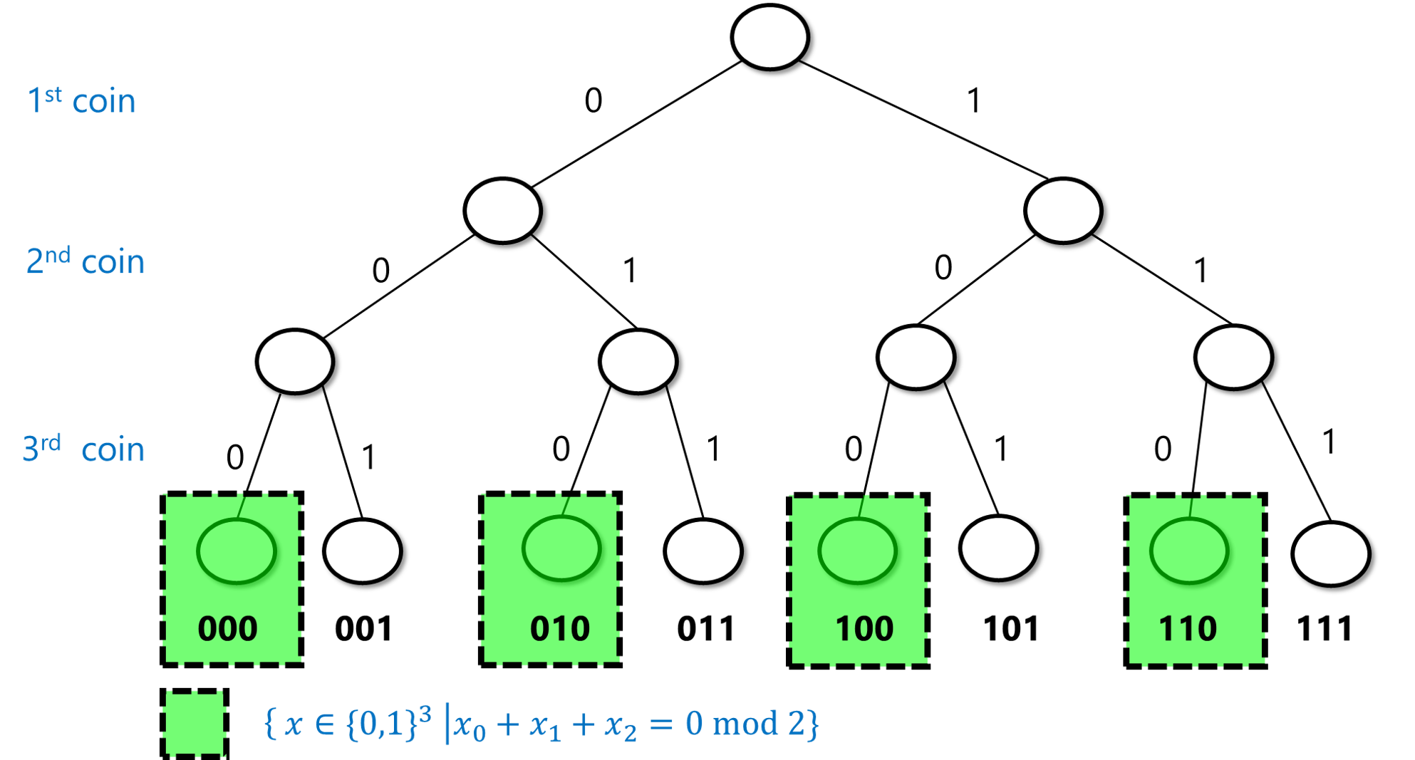
If instead of “heads” and “tails” we encode the sides of each coin by “zero” and “one”, we can encode the result of tossing $n$ coins as a string in $\{0,1\}^n$. Each particular outcome $x\in \{0,1\}^n$ is obtained with probability $2^{-n}$. For example, if we toss three coins, then we obtain each of the 8 outcomes $000,001,010,011,100,101,110,111$ with probability $2^{-3}=1/8$ (see also Figure 1). We can describe the experiment of tossing $n$ coins as choosing a string $x$ uniformly at random from $\{0,1\}^n$, and hence we’ll use the shorthand $x\sim \{0,1\}^n$ for $x$ that is chosen according to this experiment.

1: The probabilistic experiment of tossing three coins corresponds to making $2\times 2 \times 2 = 8$ choices, each with equal probability. In this example, the blue set corresponds to the event $A = \{ x\in \{0,1\}^3 \;|\; x_0 = 0 \}$ where the first coin toss is equal to $0$, and the pink set corresponds to the event $B = \{ x\in \{0,1\}^3 \;|\; x_1 = 1 \}$ where the second coin toss is equal to $1$ (with their intersection having a purplish color). As we can see, each of these events contains $4$ elements (out of $8$ total) and so has probability $1/2$. The intersection of $A$ and $B$ contains two elements, and so the probability that both of these events occur is $2/8 = 1/4$.

An event is simply a subset $A$ of $\{0,1\}^n$. The probability of $A$, denoted by $\Pr_{x\sim \{0,1\}^n}[A]$ (or $\Pr[A]$ for short, when the sample space is understood from the context), is the probability that an $x$ chosen uniformly at random will be contained in $A$. Note that this is the same as $|A|/2^n$ (where $|A|$ as usual denotes the number of elements in the set $A$). For example, the probability that $x$ has an even number of ones is $\Pr[A]$ where $A=\{ x : \sum_{i=0}^{n-1} x_i \;= 0 \mod 2 \}$. In the case $n=3$, $A=\{ 000,011,101,110 \}$, and hence $\Pr[A]=\tfrac{4}{8}=\tfrac{1}{2}$ (see Figure 2). It turns out this is true for every $n$:

2: The event that if we toss three coins $x_0,x_1,x_2 \in \{0,1\}$ then the sum of the $x_i$’s is even has probability $1/2$ since it corresponds to exactly $4$ out of the $8$ possible strings of length $3$.

For every $n>0$,

\[\Pr_{x\sim \{0,1\}^n}[ \text{$\sum_{i=0}^{n-1} x_i$ is even }] = 1/2\]

To test your intuition on probability, try to stop here and prove the lemma on your own.

We prove the lemma by induction on $n$. For the case $n=1$ it is clear since $x=0$ is even and $x=1$ is odd, and hence the probability that $x\in \{0,1\}$ is even is $1/2$. Let $n>1$. We assume by induction that the lemma is true for $n-1$ and we will prove it for $n$. We split the set $\{0,1\}^n$ into four disjoint sets $E_0,E_1,O_0,O_1$, where for $b\in \{0,1\}$, $E_b$ is defined as the set of $x\in \{0,1\}^n$ such that $x_0\cdots x_{n-2}$ has even number of ones and $x_{n-1}=b$ and similarly $O_b$ is the set of $x\in \{0,1\}^n$ such that $x_0 \cdots x_{n-2}$ has odd number of ones and $x_{n-1}=b$. Since $E_0$ is obtained by simply extending $n-1$-length string with even number of ones by the digit $0$, the size of $E_0$ is simply the number of such $n-1$-length strings which by the induction hypothesis is $2^{n-1}/2 = 2^{n-2}$. The same reasoning applies for $E_1$, $O_0$, and $O_1$. Hence each one of the four sets $E_0,E_1,O_0,O_1$ is of size $2^{n-2}$. Since $x\in \{0,1\}^n$ has an even number of ones if and only if $x \in E_0 \cup O_1$ (i.e., either the first $n-1$ coordinates sum up to an even number and the final coordinate is $0$ or the first $n-1$ coordinates sum up to an odd number and the final coordinate is $1$), we get that the probability that $x$ satisfies this property is

\[ \tfrac{|E_0\cup O_1|}{2^n} = \frac{2^{n-2}+2^{n-2}}{2^n} = \frac{1}{2} \;, \]

using the fact that $E_0$ and $O_1$ are disjoint and hence $|E_0 \cup O_1| = |E_0|+|O_1|$.

We can also use the intersection ($\cap$) and union ($\cup$) operators to talk about the probability of both event $A$ and event $B$ happening, or the probability of event $A$ or event $B$ happening. For example, the probability $p$ that $x$ has an even number of ones and $x_0=1$ is the same as $\Pr[A\cap B]$ where $A=\{ x\in \{0,1\}^n : \sum_{i=0}^{n-1} x_i =0 \mod 2 \}$ and $B=\{ x\in \{0,1\}^n : x_0 = 1 \}$. This probability is equal to $1/4$ for $n > 1$. (It is a great exercise for you to pause here and verify that you understand why this is the case.)

Because intersection corresponds to considering the logical AND of the conditions that two events happen, while union corresponds to considering the logical OR, we will sometimes use the $\wedge$ and $\vee$ operators instead of $\cap$ and $\cup$, and so write this probability $p=\Pr[A \cap B]$ defined above also as

\[ \Pr_{x\sim \{0,1\}^n} \left[ \sum_i x_i =0 \mod 2 \; \wedge \; x_0 = 1 \right] \;. \]

If $A \subseteq \{0,1\}^n$ is an event, then $\overline{A} = \{0,1\}^n \setminus A$ corresponds to the event that $A$ does not happen. Since $|\overline{A}|=2^n-|A|$, we get that

\[\Pr[\overline{A}] = \tfrac{|\overline{A}|}{2^n} = \tfrac{2^n-|A|}{2^n}=1-\tfrac{|A|}{2^n} = 1- \Pr[A] \]

This makes sense: since $A$ happens if and only if $\overline{A}$ does not happen, the probability of $\overline{A}$ should be one minus the probability of $A$.

While the above definition might seem very simple and almost trivial, the human mind seems not to have evolved for probabilistic reasoning, and it is surprising how often people can get even the simplest settings of probability wrong. One way to make sure you don’t get confused when trying to calculate probability statements is to always ask yourself the following two questions: (1) Do I understand what is the sample space that this probability is taken over?, and (2) Do I understand what is the definition of the event that we are analyzing?.

For example, suppose that I were to randomize seating in my course, and then it turned out that students sitting in row 7 performed better on the final: how surprising should we find this? If we started out with the hypothesis that there is something special about the number 7 and chose it ahead of time, then the event that we are discussing is the event $A$ that students sitting in number 7 had better performance on the final, and we might find it surprising. However, if we first looked at the results and then chose the row whose average performance is best, then the event we are discussing is the event $B$ that there exists some row where the performance is higher than the overall average. $B$ is a superset of $A$, and its probability (even if there is no correlation between sitting and performance) can be quite significant.

Random variables

Events correspond to Yes/No questions, but often we want to analyze finer questions. For example, if we make a bet at the roulette wheel, we don’t want to just analyze whether we won or lost, but also how much we’ve gained. A (real valued) random variable is simply a way to associate a number with the result of a probabilistic experiment. Formally, a random variable is a function $X:\{0,1\}^n \rightarrow \R$ that maps every outcome $x\in \{0,1\}^n$ to an element $X(x) \in \R$. For example, the function $sum:\{0,1\}^n \rightarrow \R$ that maps $x$ to the sum of its coordinates (i.e., to $\sum_{i=0}^{n-1} x_i$) is a random variable.

The expectation of a random variable $X$, denoted by $\E[X]$, is the average value that that this number takes, taken over all draws from the probabilistic experiment. In other words, the expectation of $X$ is defined as follows:

\[ \E[X] = \sum_{x\in \{0,1\}^n} 2^{-n}X(x) \;. \]

If $X$ and $Y$ are random variables, then we can define $X+Y$ as simply the random variable that maps a point $x\in \{0,1\}^n$ to $X(x)+Y(x)$. One basic and very useful property of the expectation is that it is linear:

\[ \E[ X+Y ] = \E[X] + \E[Y] \]

\[ \begin{gathered} \E [X+Y] = \sum_{x\in \{0,1\}^n}2^{-n}\left(X(x)+Y(x)\right) = \\ \sum_{x\in \{0,1\}^b} 2^{-n}X(x) + \sum_{x\in \{0,1\}^b} 2^{-n}Y(x) = \\ \E[X] + \E[Y] \end{gathered} \]

Similarly, $\E[kX] = k\E[X]$ for every $k \in \R$. For example, using the linearity of expectation, it is very easy to show that the expectation of the sum of the $x_i$’s for $x \sim \{0,1\}^n$ is equal to $n/2$. Indeed, if we write $X= \sum_{i=0}^{n-1} x_i$ then $X= X_0 + \cdots + X_{n-1}$ where $X_i$ is the random variable $x_i$. Since for every $i$, $\Pr[X_i=0] = 1/2$ and $\Pr[X_i=1]=1/2$, we get that $\E[X_i] = (1/2)\cdot 0 + (1/2)\cdot 1 = 1/2$ and hence $\E[X] = \sum_{i=0}^{n-1}\E[X_i] = n\cdot(1/2) = n/2$.

If you have not seen discrete probability before, please go over this argument again until you are sure you follow it; it is a prototypical simple example of the type of reasoning we will employ again and again in this course.

If $A$ is an event, then $1_A$ is the random variable such that $1_A(x)$ equals $1$ if $x\in A$, and $1_A(x)=0$ otherwise. Note that $\Pr[A] = \E[1_A]$ (can you see why?). Using this and the linearity of expectation, we can show one of the most useful bounds in probability theory:

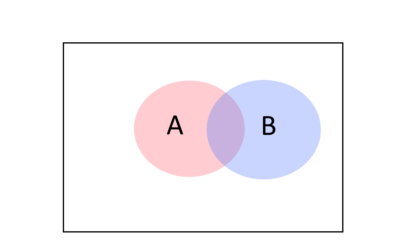
For every two events $A,B$, $\Pr[ A \cup B] \leq \Pr[A]+\Pr[B]$

Before looking at the proof, try to see why the union bound makes intuitive sense. We can also prove it directly from the definition of probabilities and the cardinality of sets, together with the equation $|A \cup B| \leq |A|+|B|$. Can you see why the latter equation is true? (See also Figure 3.)

For every $x$, the variable $1_{A\cup B}(x) \leq 1_A(x)+1_B(x)$. Hence, $\Pr[A\cup B] = \E[ 1_{A \cup B} ] \leq \E[1_A+1_B] = \E[1_A]+\E[1_B] = \Pr[A]+\Pr[B]$.

The way we often use this in theoretical computer science is to argue that, for example, if there is a list of 100 bad events that can happen, and each one of them happens with probability at most $1/10000$, then with probability at least $1-100/10000 = 0.99$, no bad event happens.

3: The *union bound* tells us that the probability of $A$ or $B$ happening is at most the sum of the individual probabilities. We can see it by noting that for every two sets $|A\cup B| \leq |A|+|B|$ (with equality only if $A$ and $B$ have no intersection).

Distributions over strings

While most of the time we think of random variables as having as output a real number, we sometimes consider random variables whose output is a string. That is, we can think of a map $Y:\{0,1\}^n \rightarrow \{0,1\}^*$ and consider the “random variable” $Y$ such that for every $y\in \{0,1\}^*$, the probability that $Y$ outputs $y$ is equal to $\tfrac{1}{2^n}\left| \{ x \in \{0,1\}^n \;|\; Y(x)=y \}\right|$. To avoid confusion, we will typically refer to such string-valued random variables as distributions over strings. So, a distribution $Y$ over strings $\{0,1\}^*$ can be thought of as a finite collection of strings $y_0,\ldots,y_{M-1} \in \{0,1\}^*$ and probabilities $p_0,\ldots,p_{M-1}$ (which are non-negative numbers summing up to one), so that $\Pr[ Y = y_i ] = p_i$.

Two distributions $Y$ and $Y'$ are identical if they assign the same probability to every string. For example, consider the following two functions $Y,Y':\{0,1\}^2 \rightarrow \{0,1\}^2$. For every $x \in \{0,1\}^2$, we define $Y(x)=x$ and $Y'(x)=x_0(x_0\oplus x_1)$ where $\oplus$ is the XOR operations. Although these are two different functions, they induce the same distribution over $\{0,1\}^2$ when invoked on a uniform input. The distribution $Y(x)$ for $x\sim \{0,1\}^2$ is of course the uniform distribution over $\{0,1\}^2$. On the other hand $Y'$ is simply the map $00 \mapsto 00$, $01 \mapsto 01$, $10 \mapsto 11$, $11 \mapsto 10$ which is a permutation over the map $F:\{0,1\}^2 \rightarrow \{0,1\}^2$ defined as $F(x_0x_1)=x_0x_1$ and the map $G:\{0,1\}^2 \rightarrow \{0,1\}^2$ defined as $G(x_0x_1)=x_0(x_0 \oplus x_1)$

More general sample spaces.

While in this chapter we assume that the underlying probabilistic experiment corresponds to tossing $n$ independent coins, everything we say easily generalizes to sampling $x$ from a more general finite or countable set $S$ (and not-so-easily generalizes to uncountable sets $S$ as well). A probability distribution over a finite set $S$ is simply a function $\mu : S \rightarrow [0,1]$ such that $\sum_{x\in S}\mu(s)=1$. We think of this as the experiment where we obtain every $x\in S$ with probability $\mu(s)$, and sometimes denote this as $x\sim \mu$. An event $A$ is a subset of $S$, and the probability of $A$, which we denote by $\Pr_\mu[A]$, is $\sum_{x\in A} \mu(x)$. A random variable is a function $X:S \rightarrow \R$, where the probability that $X=y$ is equal to $\sum_{x\in S \text{ s.t. } X(x)=y} \mu(x)$.

Correlations and independence

One of the most delicate but important concepts in probability is the notion of independence (and the opposing notion of correlations). Subtle correlations are often behind surprises and errors in probability and statistical analysis, and several mistaken predictions have been blamed on miscalculating the correlations between, say, housing prices in Florida and Arizona, or voter preferences in Ohio and Michigan. See also Joe Blitzstein’s aptly named talk “Conditioning is the Soul of Statistics”. (Another thorny issue is of course the difference between correlation and causation. Luckily, this is another point we don’t need to worry about in our clean setting of tossing $n$ coins.)

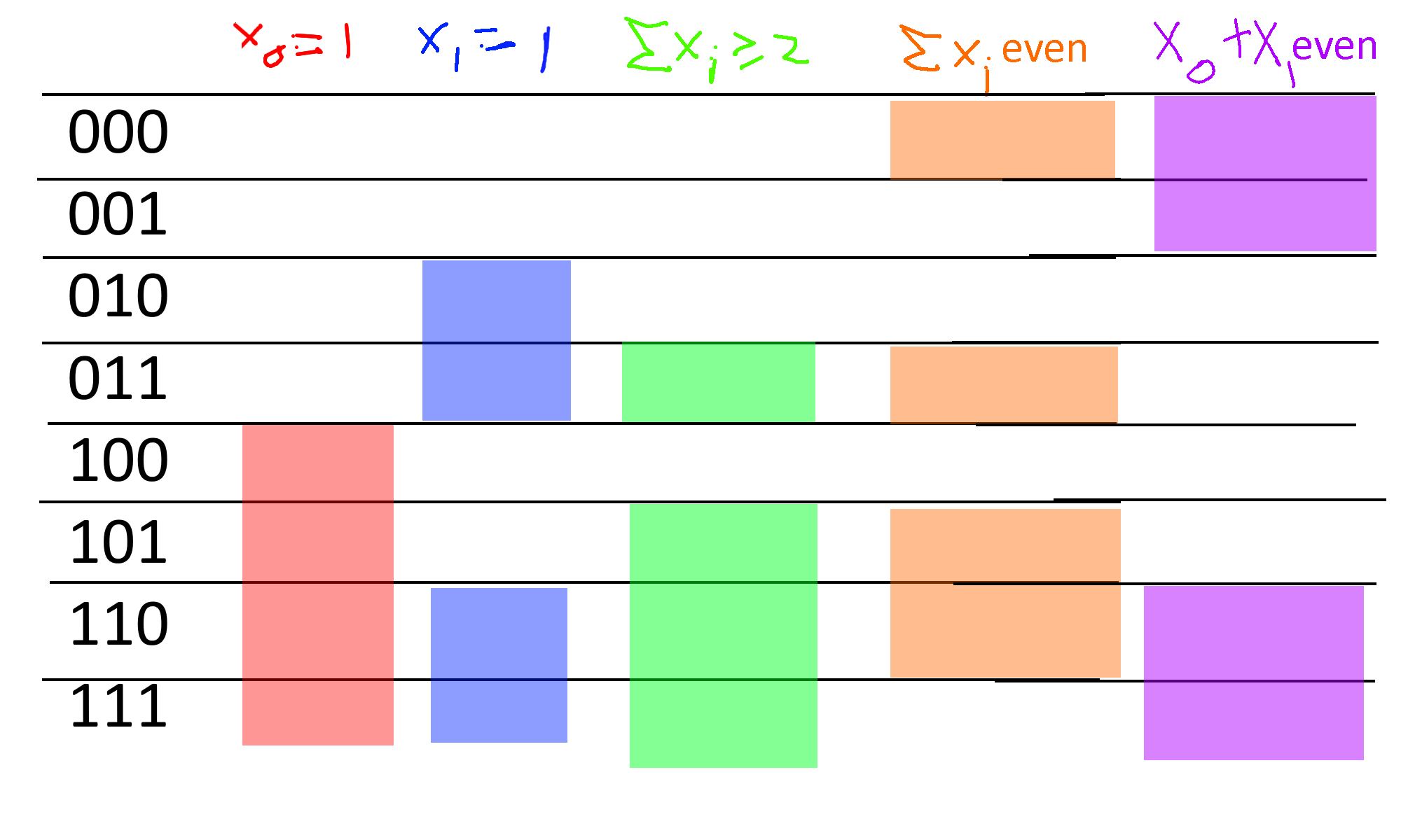
Two events $A$ and $B$ are independent if the fact that $A$ happens makes $B$ neither more nor less likely to happen. For example, if we think of the experiment of tossing $3$ random coins $x\in \{0,1\}^3$, and we let $A$ be the event that $x_0=1$ and $B$ the event that $x_0 + x_1 + x_2 \geq 2$, then if $A$ happens it is more likely that $B$ happens, and hence these events are not independent. On the other hand, if we let $C$ be the event that $x_1=1$, then because the second coin toss is not affected by the result of the first one, the events $A$ and $C$ are independent.

The formal definition is that events $A$ and $B$ are independent if $\Pr[A \cap B]=\Pr[A] \cdot \Pr[B]$. If $\Pr[A \cap B] > \Pr[A]\cdot \Pr[B]$ then we say that $A$ and $B$ are positively correlated, while if $\Pr[ A \cap B] < \Pr[A] \cdot \Pr[B]$ then we say that $A$ and $B$ are negatively correlated (see Figure 1).

4: Two events $A$ and $B$ are *independent* if $\Pr[A \cap B]=\Pr[A]\cdot \Pr[B]$. In the two figures above, the empty $x\times x$ square is the sample space, and $A$ and $B$ are two events in this sample space. In the left figure, $A$ and $B$ are independent, while in the right figure they are negatively correlated, since $B$ is less likely to occur if we condition on $A$ (and vice versa). Mathematically, one can see this by noticing that in the left figure the areas of $A$ and $B$ respectively are $a\cdot x$ and $b\cdot x$, and so their probabilities are $\tfrac{a\cdot x}{x^2}=\tfrac{a}{x}$ and $\tfrac{b\cdot x}{x^2}=\tfrac{b}{x}$ respectively, while the area of $A \cap B$ is $a\cdot b$ which corresponds to the probability $\tfrac{a\cdot b}{x^2}$. In the right figure, the area of the triangle $B$ is $\tfrac{b\cdot x}{2}$ which corresponds to a probability of $\tfrac{b}{2x}$, but the area of $A \cap B$ is $\tfrac{b' \cdot a}{2}$ for some $b'<b$. This means that the probability of $A \cap B$ is $\tfrac{b'\cdot a}{2x^2} < \tfrac{b}{2x} \cdot \tfrac{a}{x}$, or in other words $\Pr[A \cap B ] < \Pr[A] \cdot \Pr[B]$.

If we consider the above examples on the experiment of choosing $x\in \{0,1\}^3$ then we can see that

\[ \begin{aligned} \Pr[x_0=1] &= \tfrac{1}{2} \\ \Pr[x_0+x_1+x_2 \geq 2] = \Pr[\{ 011,101,110,111 \}] &= \tfrac{4}{8} = \tfrac{1}{2} \end{aligned} \]

but

\[ \Pr[x_0 =1 \; \wedge \; x_0+x_1+x_2 \geq 2 ] = \Pr[ \{101,110,111 \} ] = \tfrac{3}{8} > \tfrac{1}{2} \cdot \tfrac{1}{2} \]

and hence, as we already observed, the events $\{ x_0 = 1 \}$ and $\{ x_0+x_1+x_2 \geq 2 \}$ are not independent and in fact are positively correlated. On the other hand, $\Pr[ x_0 = 1 \wedge x_1 = 1 ] = \Pr[ \{110,111 \}] = \tfrac{2}{8} = \tfrac{1}{2} \cdot \tfrac{1}{2}$ and hence the events $\{x_0 = 1 \}$ and $\{ x_1 = 1 \}$ are indeed independent.

People sometimes confuse the notion of disjointness and independence, but these are actually quite different. Two events $A$ and $B$ are disjoint if $A \cap B = \emptyset$, which means that if $A$ happens then $B$ definitely does not happen. They are independent if $\Pr[A \cap B]=\Pr[A]\Pr[B]$ which means that knowing that $A$ happens gives us no information about whether $B$ happened or not. If $A$ and $B$ have nonzero probability, then being disjoint implies that they are not independent, since in particular it means that they are negatively correlated.

Conditional probability: If $A$ and $B$ are events, and $A$ happens with nonzero probability then we define the probability that $B$ happens conditioned on $A$ to be $\Pr[B|A] = \Pr[A \cap B]/\Pr[A]$. This corresponds to calculating the probability that $B$ happens if we already know that $A$ happened. Note that $A$ and $B$ are independent if and only if $\Pr[B|A]=\Pr[B]$.

More than two events: We can generalize this definition to more than two events. We say that events $A_1,\ldots,A_k$ are mutually independent if knowing that any set of them occurred or didn’t occur does not change the probability that an event outside the set occurs. Formally, the condition is that for every subset $I \subseteq [k]$,

\[ \Pr[ \wedge_{i\in I} A_i] =\prod_{i\in I} \Pr[A_i]. \]

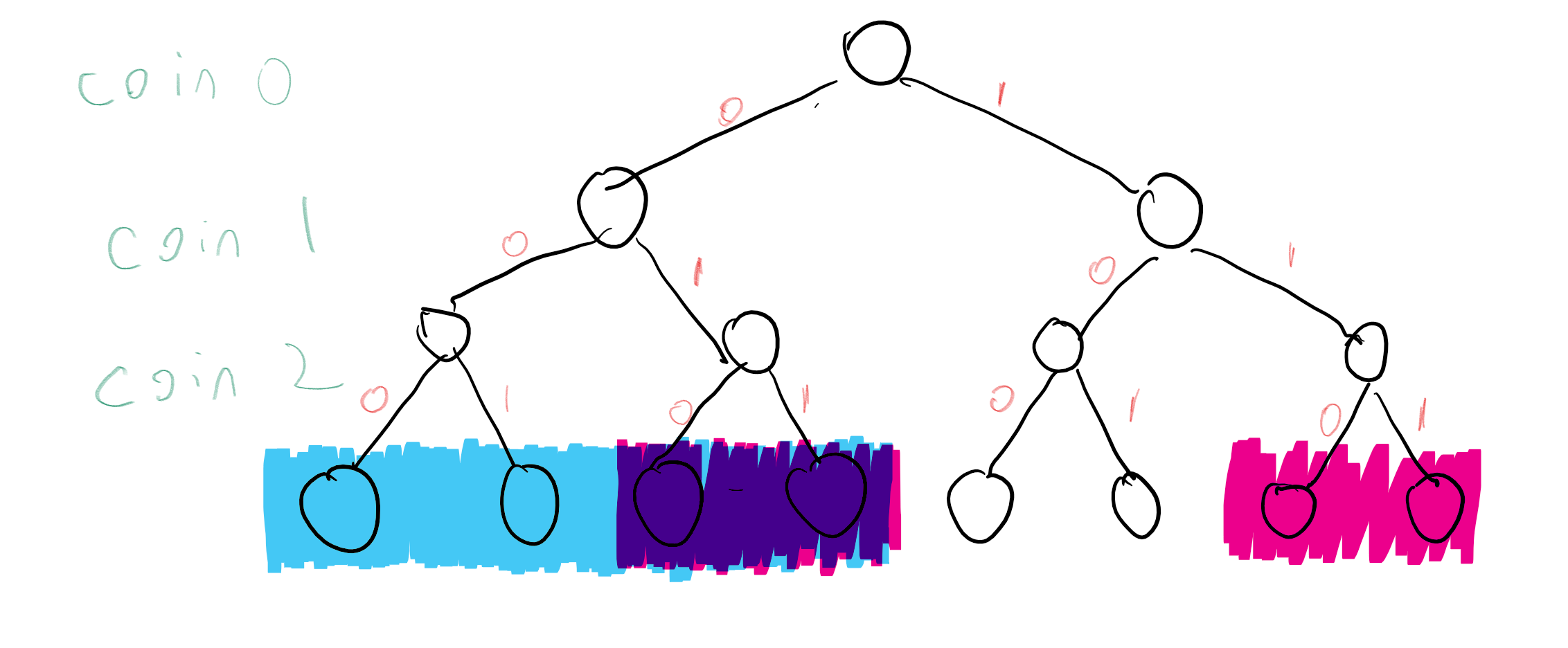
For example, if $x\sim \{0,1\}^3$, then the events $\{ x_0=1 \}$, $\{ x_1 = 1\}$ and $\{x_2 = 1 \}$ are mutually independent. On the other hand, the events $\{x_0 = 1 \}$, $\{x_1 = 1\}$ and $\{ x_0 + x_1 = 0 \mod 2 \}$ are not mutually independent, even though every pair of these events is independent (can you see why? see also Figure 5).

5: Consider the sample space $\{0,1\}^n$ and the events $A,B,C,D,E$ corresponding to $A$: $x_0=1$, $B$: $x_1=1$, $C$: $x_0+x_1+x_2 \geq 2$, $D$: $x_0+x_1+x_2 = 0 mod 2$ and $D$: $x_0+x_1 = 0 mod 2$. We can see that $A$ and $B$ are independent, $C$ is positively correlated with $A$ and positively correlated with $B$, the three events $A,B,D$ are mutually independent, and while every pair out of $A,B,E$ is independent, the three events $A,B,E$ are not mutually independent since their intersection has probability $\tfrac{2}{8}=\tfrac{1}{4}$ instead of $\tfrac{1}{2}\cdot \tfrac{1}{2} \cdot \tfrac{1}{2} = \tfrac{1}{8}$.

Independent random variables

We say that two random variables $X:\{0,1\}^n \rightarrow \R$ and $Y:\{0,1\}^n \rightarrow \R$ are independent if for every $u,v \in \R$, the events $\{ X=u \}$ and $\{ Y=v \}$ are independent. (We use $\{ X=u \}$ as shorthand for $\{ x \;|\; X(x)=u \}$.) In other words, $X$ and $Y$ are independent if $\Pr[ X=u \wedge Y=v]=\Pr[X=u]\Pr[Y=v]$ for every $u,v \in \R$. For example, if two random variables depend on the result of tossing different coins then they are independent:

Suppose that $S=\{ s_0,\ldots, s_{k-1} \}$ and $T=\{ t_0 ,\ldots, t_{m-1} \}$ are disjoint subsets of $\{0,\ldots,n-1\}$ and let $X,Y:\{0,1\}^n \rightarrow \R$ be random variables such that $X=F(x_{s_0},\ldots,x_{s_{k-1}})$ and $Y=G(x_{t_0},\ldots,x_{t_{m-1}})$ for some functions $F: \{0,1\}^k \rightarrow \R$ and $G: \{0,1\}^m \rightarrow \R$. Then $X$ and $Y$ are independent.

The notation in the lemma’s statement is a bit cumbersome, but at the end of the day, it simply says that if $X$ and $Y$ are random variables that depend on two disjoint sets $S$ and $T$ of coins (for example, $X$ might be the sum of the first $n/2$ coins, and $Y$ might be the largest consecutive stretch of zeroes in the second $n/2$ coins), then they are independent.

Let $a,b\in \R$, and let $A = \{ x \in \{0,1\}^k : F(x)=a \}$ and $B=\{ x\in \{0,1\}^m : G(x)=b \}$. Since $S$ and $T$ are disjoint, we can reorder the indices so that $S = \{0,\ldots,k-1\}$ and $T=\{k,\ldots,k+m-1\}$ without affecting any of the probabilities. Hence we can write $\Pr[X=a \wedge Y=b] = |C|/2^n$ where $C= \{ x_0,\ldots,x_{n-1} : (x_0,\ldots,x_{k-1}) \in A \wedge (x_k,\ldots,x_{k+m-1}) \in B \}$. Another way to write this using string concatenation is that $C = \{ xyz : x\in A, y\in B, z\in \{0,1\}^{n-k-m} \}$, and hence $|C|=|A||B|2^{n-k-m}$, which means that

\[ \tfrac{|C|}{2^n} = \tfrac{|A|}{2^k}\tfrac{|B|}{2^m}\tfrac{2^{n-k-m}}{2^{n-k-m}}=\Pr[X=a]\Pr[Y=b] . \]

Note that if $X$ and $Y$ are independent random variables then (if we let $S_X,S_Y$ denote all the numbers that have positive probability of being the output of $X$ and $Y$, respectively) it holds that:

\[ \begin{gathered} \E[ \ensuremath{\mathit{XY}} ] = \sum_{a \in S_X,b \in S_Y} {\textstyle\Pr[X=a \wedge Y=b]}\cdot ab \; =^{(1)} \; \sum_{a \in S_X,b \in S_Y} {\textstyle \Pr[X=a]\Pr[Y=b]}\cdot ab =^{(2)} \\ \left(\sum_{a \in S_X} {\textstyle \Pr[X=a]}\cdot a\right)\left(\sum_{b \in S_Y} {\textstyle \Pr[Y=b]}b\right) =^{(3)} \\ \E[X] \E[Y] \end{gathered} \]

where the first equality ($=^{(1)}$) follows from the independence of $X$ and $Y$, the second equality ($=^{(2)}$) follows by “opening the parentheses” of the righthand side, and the third inequality ($=^{(3)}$) follows from the definition of expectation. (This is not an “if and only if”; see Exercise 0.8.)

Another useful fact is that if $X$ and $Y$ are independent random variables, then so are $F(X)$ and $G(Y)$ for all functions $F,G:\R \rightarrow R$. This is intuitively true since learning $F(X)$ can only provide us with less information than does learning $X$ itself. Hence, if learning $X$ does not teach us anything about $Y$ (and so also about $F(Y)$) then neither will learning $F(X)$. Indeed, to prove this we can write for every $a,b \in \R$:

\[ \begin{gathered} \Pr[ F(X)=a \wedge G(Y)=b ] = \sum_{x \text{ s.t.} F(x)=a, y \text{ s.t. } G(y)=b} \Pr[ X=x \wedge Y=y ] = \\ \sum_{x \text{ s.t.} F(x)=a, y \text{ s.t. } G(y)=b} \Pr[ X=x ] \Pr[ Y=y ] = \\ \left( \sum_{x \text{ s.t.} F(x)=a } \Pr[X=x ] \right) \cdot \left( \sum_{y \text{ s.t.} G(y)=b } \Pr[Y=y ] \right) = \\ \Pr[ F(X)=a] \Pr[G(Y)=b] . \end{gathered} \]

Collections of independent random variables.

We can extend the notions of independence to more than two random variables: we say that the random variables $X_0,\ldots,X_{n-1}$ are mutually independent if for every $a_0,\ldots,a_{n-1} \in \R$,

\[ \Pr\left[X_0=a_0 \wedge \cdots \wedge X_{n-1}=a_{n-1}\right]=\Pr[X_0=a_0]\cdots \Pr[X_{n-1}=a_{n-1}] . \]

And similarly, we have that

If $X_0,\ldots,X_{n-1}$ are mutually independent then

\[ \E[ \prod_{i=0}^{n-1} X_i ] = \prod_{i=0}^{n-1} \E[X_i] . \]

If $X_0,\ldots,X_{n-1}$ are mutually independent, and $Y_0,\ldots,Y_{n-1}$ are defined as $Y_i = F_i(X_i)$ for some functions $F_0,\ldots,F_{n-1}:\R \rightarrow \R$, then $Y_0,\ldots,Y_{n-1}$ are mutually independent as well.

We leave proving Lemma 0.10 and Lemma 0.11 as Exercise 0.9 Exercise 0.10. It is good idea for you stop now and do these exercises to make sure you are comfortable with the notion of independence, as we will use it heavily later on in this course.

Concentration and tail bounds

The name “expectation” is somewhat misleading. For example, suppose that you and I place a bet on the outcome of 10 coin tosses, where if they all come out to be $1$’s then I pay you 100,000 dollars and otherwise you pay me 10 dollars. If we let $X:\{0,1\}^{10} \rightarrow \R$ be the random variable denoting your gain, then we see that

\[ \E[X] = 2^{-10}\cdot 100000 - (1-2^{-10})10 \sim 90 . \]

But we don’t really “expect” the result of this experiment to be for you to gain 90 dollars. Rather, 99.9% of the time you will pay me 10 dollars, and you will hit the jackpot 0.01% of the times.

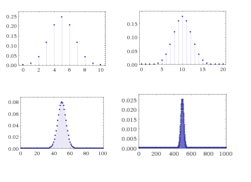
However, if we repeat this experiment again and again (with fresh and hence independent coins), then in the long run we do expect your average earning to be close to 90 dollars, which is the reason why casinos can make money in a predictable way even though every individual bet is random. For example, if we toss $n$ independent and unbiased coins, then as $n$ grows, the number of coins that come up ones will be more and more concentrated around $n/2$ according to the famous “bell curve” (see Figure 6).

6: The probabilities that we obtain a particular sum when we toss $n=10,20,100,1000$ coins converge quickly to the Gaussian/normal distribution.

Much of probability theory is concerned with so called concentration or tail bounds, which are upper bounds on the probability that a random variable $X$ deviates too much from its expectation. The first and simplest one of them is Markov’s inequality:

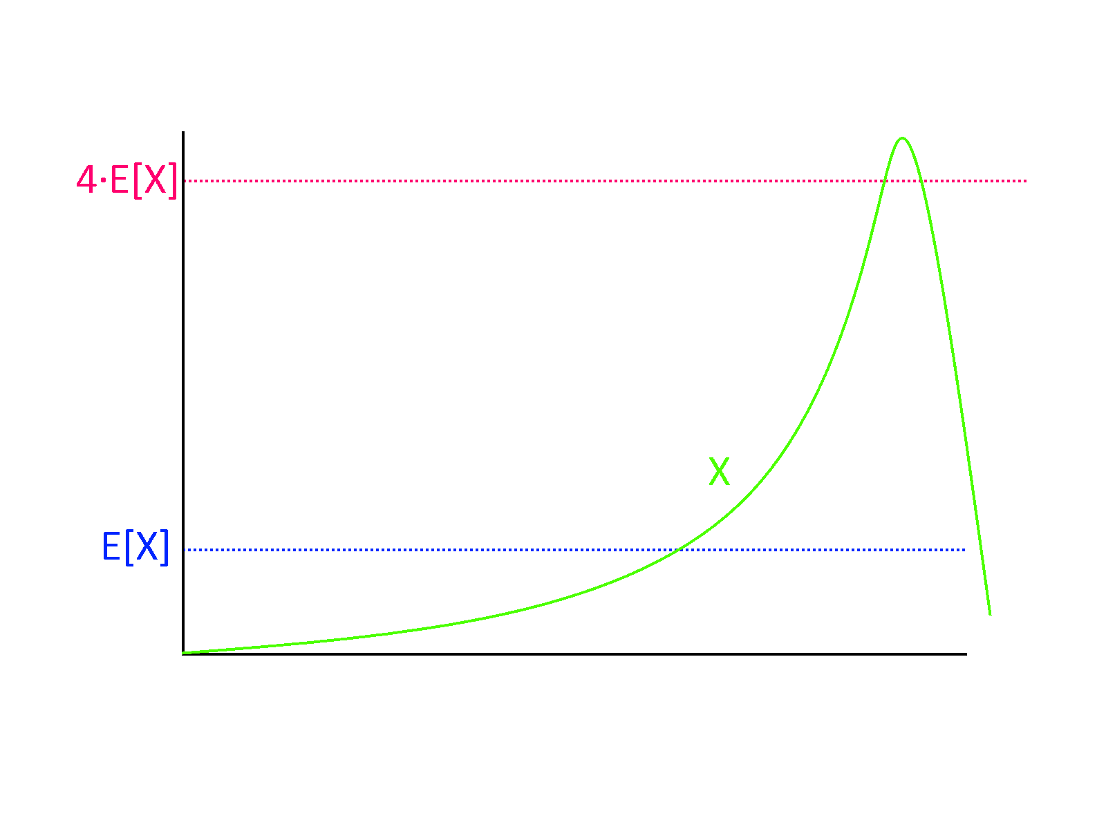
If $X$ is a non-negative random variable then $\Pr[ X \geq k \E[X] ] \leq 1/k$.

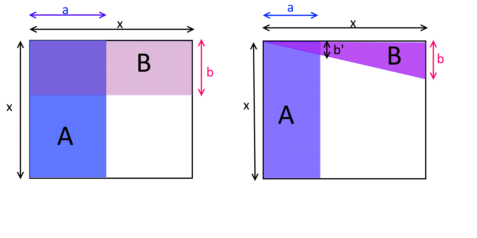
Markov’s Inequality is actually a very natural statement (see also Figure 7). For example, if you know that the average (not the median!) household income in the US is 70,000 dollars, then in particular you can deduce that at most 25 percent of households make more than 280,000 dollars, since otherwise, even if the remaining 75 percent had zero income, the top 25 percent alone would cause the average income to be larger than 70,000 dollars. From this example you can already see that in many situations, Markov’s inequality will not be tight and the probability of deviating from expectation will be much smaller: see the Chebyshev and Chernoff inequalities below.

Let $\mu = \E[X]$ and define $Y=1_{X \geq k \mu}$. That is, $Y(x)=1$ if $X(x) \geq k \mu$ and $Y(x)=0$ otherwise. Note that by definition, for every $x$, $Y(x) \leq X/(k\mu)$. We need to show $\E[Y] \leq 1/k$. But this follows since $\E[Y] \leq \E[X/k(\mu)] = \E[X]/(k\mu) = \mu/(k\mu)=1/k$.

7: Markov’s Inequality tells us that a non-negative random variable $X$ cannot be much larger than its expectation, with high probability. For example, if the expectation of $X$ is $\mu$, then the probability that $X>4\mu$ must be at most $1/4$, as otherwise just the contribution from this part of the sample space will be too large.

Going beyond Markov’s Inequality: Markov’s inequality says that a (non-negative) random variable $X$ can’t go too crazy and be, say, a million times its expectation, with significant probability. But ideally we would like to say that with high probability, $X$ should be very close to its expectation, e.g., in the range $[0.99 \mu, 1.01 \mu]$ where $\mu = \E[X]$. This is not generally true, but does turn out to hold when $X$ is obtained by combining (e.g., adding) many independent random variables. This phenomenon, variants of which are known as “law of large numbers”, “central limit theorem”, “invariance principles” and “Chernoff bounds”, is one of the most fundamental in probability and statistics, and is one that we heavily use in computer science as well.

Chebyshev’s Inequality

A standard way to measure the deviation of a random variable from its expectation is by using its standard deviation. For a random variable $X$, we define the variance of $X$ as $\mathrm{Var}[X] = \E[(X-\mu)^2]$ where $\mu = \E[X]$; i.e., the variance is the average squared distance of $X$ from its expectation. The standard deviation of $X$ is defined as $\sigma[X] = \sqrt{\mathrm{Var}[X]}$. (This is well-defined since the variance, being an average of a square, is always a non-negative number.)

Using Chebyshev’s inequality, we can control the probability that a random variable is too many standard deviations away from its expectation.

Suppose that $\mu=\E[X]$ and $\sigma^2 = \mathrm{Var}[X]$. Then for every $k>0$, $\Pr[ |X-\mu | \geq k \sigma ] \leq 1/k^2$.

The proof follows from Markov’s inequality. We define the random variable $Y = (X-\mu)^2$. Then $\E[Y] = \mathrm{Var}[X] = \sigma^2$, and hence by Markov the probability that $Y > k^2\sigma^2$ is at most $1/k^2$. But clearly $(X-\mu)^2 \geq k^2\sigma^2$ if and only if $|X-\mu| \geq k\sigma$.

One example of how to use Chebyshev’s inequality is the setting when $X = X_1 + \cdots + X_n$ where $X_i$’s are independent and identically distributed (i.i.d for short) variables with values in $[0,1]$ where each has expectation $1/2$. Since $\E[X] = \sum_i \E[X_i] = n/2$, we would like to say that $X$ is very likely to be in, say, the interval $[0.499n,0.501n]$. Using Markov’s inequality directly will not help us, since it will only tell us that $X$ is very likely to be at most $100n$ (which we already knew, since it always lies between $0$ and $n$). However, since $X_1,\ldots,X_n$ are independent,

\[ \mathrm{Var}[X_1+\cdots +X_n] = \mathrm{Var}[X_1]+\cdots + \mathrm{Var}[X_n] \;\;(1)\;. \]

(We leave showing this to the reader as Exercise 0.11.)

For every random variable $X_i$ in $[0,1]$, $\mathrm{Var}[X_i] \leq 1$ (if the variable is always in $[0,1]$, it can’t be more than $1$ away from its expectation), and hence Equation 1 implies that $\mathrm{Var}[X]\leq n$ and hence $\sigma[X] \leq \sqrt{n}$. For large $n$, $\sqrt{n} \ll 0.001n$, and in particular if $\sqrt{n} \leq 0.001n/k$, we can use Chebyshev’s inequality to bound the probability that $X$ is not in $[0.499n,0.501n]$ by $1/k^2$.

The Chernoff bound

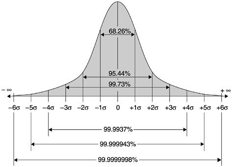
Chebyshev’s inequality already shows a connection between independence and concentration, but in many cases we can hope for a quantitatively much stronger result. If, as in the example above, $X= X_1+\ldots+X_n$ where the $X_i$’s are bounded i.i.d random variables of mean $1/2$, then as $n$ grows, the distribution of $X$ would be roughly the normal or Gaussian distribution$-$ that is, distributed according to the bell curve (see Figure 6 and Figure 8). This distribution has the property of being very concentrated in the sense that the probability of deviating $k$ standard deviations from the mean is not merely $1/k^2$ as is guaranteed by Chebyshev, but rather is roughly $e^{-k^2}$. Specifically, for a normal random variable $X$ of expectation $\mu$ and standard deviation $\sigma$, the probability that $|X-\mu| \geq k\sigma$ is at most $2e^{-k^2/2}$. That is, we have an exponential decay of the probability of deviation.

8: In the *normal distribution* or the Bell curve, the probability of deviating $k$ standard deviations from the expectation shrinks *exponentially* in $k^2$, and specifically with probability at least $1-2e^{-k^2/2}$, a random variable $X$ of expectation $\mu$ and standard deviation $\sigma$ satisfies $\mu -k\sigma \leq X \leq \mu+k\sigma$. This figure gives more precise bounds for $k=1,2,3,4,5,6$. (Image credit:Imran Baghirov)

The following extremely useful theorem shows that such exponential decay occurs every time we have a sum of independent and bounded variables. This theorem is known under many names in different communities, though it is mostly called the Chernoff bound in the computer science literature:

If $X_1,\ldots,X_n$ are i.i.d random variables such that $X_i \in [0,1]$ and $\E[X_i]=p$ for every $i$, then for every $\epsilon >0$

\[ \Pr[ \left| \sum_{i=0}^{n-1} X_i - pn \right| > \epsilon n ] \leq 2\cdot e^{-2\epsilon^2 n} . \]

We omit the proof, which appears in many texts, and uses Markov’s inequality on i.i.d random variables $Y_0,\ldots,Y_n$ that are of the form $Y_i = e^{\lambda X_i}$ for some carefully chosen parameter $\lambda$. See Exercise 0.14 for a proof of the simple (but highly useful and representative) case where each $X_i$ is $\{0,1\}$ valued and $p=1/2$. (See also Exercise 0.15 for a generalization.)

Exercises

Prove that for every finite $S,T$, there are $(|T|+1)^{|S|}$ partial functions from $S$ to $T$.

For every pair of functions $F,G$ below, determine which of the following relations holds: $F=O(G)$, $F=\Omega(G)$, $F=o(G)$ or $F=\omega(G)$.

$F(n)=n$, $G(n)=100n$.
$F(n)=n$, $G(n)=\sqrt{n}$.
$F(n)=n\log n$, $G(n)=2^{(\log (n))^2}$.
$F(n)=\sqrt{n}$, $G(n)=2^{\sqrt{\log n}}$
$F(n) = \binom{n}{\ceil{0.2 n}}$ , $G(n) = 2^{0.1 n}$ (where $\binom{n}{k}$ is the number of $k$-sized subsets of a set of size $n$) and $g(n) = 2^{0.1 n}$. See footnote for hint.²

Give an example of a pair of functions $F,G:\N \rightarrow \N$ such that neither $F=O(G)$ nor $G=O(F)$ holds.

In the following exercise $X,Y$ denote random variables over some sample space $S$. You can assume that the probability on $S$ is the uniform distribution— every point $s$ is output with probability $1/|S|$. Thus ${\mathbb{E}}[X]= (1/|S|)\sum_{s\in S}X(s)$. We define the variance and standard deviation of $X$ and $Y$ as above (e.g., $Var[X] = {\mathbb{E}}[(X-{\mathbb{E}}[X])^2 ]$ and the standard deviation is the square root of the variance). You can reuse your answers to prior questions in the later ones.

Prove that $Var[X]$ is always non-negative.
Prove that $Var[X] = {\mathbb{E}}[X^2] - {\mathbb{E}}[X]^2$.
Prove that always ${\mathbb{E}}[X^2] \geq {\mathbb{E}}[X]^2$.
Give an example for a random variable $X$ such that ${\mathbb{E}}[X^2] > {\mathbb{E}}[X]^2$.
Give an example for a random variable $X$ such that its standard deviation is not equal to ${\mathbb{E}}[ | X - {\mathbb{E}}[X] | ]$.
Give an example for a random variable $X$ such that its standard deviation is equal to to ${\mathbb{E}}[ | X - {\mathbb{E}}[X] | ]$.
Give an example for two random variables $X,Y$ such that ${\mathbb{E}}[\ensuremath{\mathit{XY}}] = {\mathbb{E}}[X]{\mathbb{E}}[Y]$.
Give an example for two random variables $X,Y$ such that ${\mathbb{E}}[\ensuremath{\mathit{XY}}] \neq {\mathbb{E}}[X]{\mathbb{E}}[Y]$.
Prove that if $X$ and $Y$ are independent random variables (i.e., for every $x,y$, $\Pr[X=x \wedge Y=y]=\Pr[X=x]\Pr[Y=y]$) then ${\mathbb{E}}[\ensuremath{\mathit{XY}}]={\mathbb{E}}[X]{\mathbb{E}}[Y]$ and $Var[X+Y]=Var[X]+Var[Y]$.

Suppose that $H$ is chosen to be a random function mapping the numbers $\{1,\ldots,n\}$ to the numbers $\{1,..,m \}$. That is, for every $i\in \{1,\ldots,n\}$, $H(i)$ is chosen to be a random number in $\{ 1,\ldots, m\}$ and that choice is done independently for every $i$. For every $i<j \in \{1,\ldots,n\}$, define the random variable $X_{i,j}$ to equal $1$ if there was a collision between $H(i)$ and $H(j)$ in the sense that $H(i)=H(j)$ and to equal $0$ otherwise.

For every $i<j$, compute ${\mathbb{E}}[ X_{i,j} ]$.
Define $Y = \sum_{i<j} X_{i,j}$ to be the total number of collisions. Compute ${\mathbb{E}}[ Y ]$ as a function of $n$ and $m$. In particular your answer should imply that if $m < n^2/1000$ then ${\mathbb{E}}[Y]>1$ and hence in expectation there should be at least one collision and so the function $H$ will not be one to one.
Prove that if $m > 1000\cdot n^2$ then the probability that $H$ is one to one is at least $0.9$.
Give an example of a random variable $Z$ (unrelated to the function $H$) that is always equal to a non-negative integer, and such that ${\mathbb{E}}[Z] \geq 1000$ but $\Pr[ Z > 0] < 0.001$.
Prove that if $m < n^2/1000$ then the probability that $H$ is one to one is at most $0.1$.

Exercises

Suppose that we toss three independent fair coins $a,b,c \in \{0,1\}$. What is the probability that the XOR of $a$,$b$, and $c$ is equal to $1$? What is the probability that the AND of these three values is equal to $1$? Are these two events independent?

Give an example of random variables $X,Y: \{0,1\}^3 \rightarrow \R$ such that $\E[\ensuremath{\mathit{XY}}] \neq \E[X]\E[Y]$.

Give an example of random variables $X,Y: \{0,1\}^3 \rightarrow \R$ such that $X$ and $Y$ are not independent but $\E[\ensuremath{\mathit{XY}}] =\E[X]\E[Y]$.

Prove Lemma 0.10

Prove Lemma 0.11

Prove that if $X_0,\ldots,X_{n-1}$ are independent random variables then $\mathrm{Var}[X_0+\cdots+X_{n-1}]=\sum_{i=0}^{n-1} \mathrm{Var}[X_i]$.

Recall the definition of a distribution $\mu$ over some finite set $S$. Shannon defined the entropy of a distribution $\mu$, denoted by $H(\mu)$, to be $\sum_{x\in S} \mu(x)\log(1/\mu(x))$. The idea is that if $\mu$ is a distribution of entropy $k$, then encoding members of $\mu$ will require $k$ bits, in an amortized sense. In this exercise we justify this definition. Let $\mu$ be such that $H(\mu)=k$.
1. Prove that for every one to one function $F:S \rightarrow \{0,1\}^*$, $\E_{x \sim \mu} |F(x)| \geq k$.
2. Prove that for every $\epsilon$, there is some $n$ and a one-to-one function $F:S^n \rightarrow \{0,1\}^*$, such that $\E_{x\sim \mu^n} |F(x)| \leq n(k+\epsilon)$, where $x \sim \mu$ denotes the experiments of choosing $x_0,\ldots,x_{n-1}$ each independently from $S$ using the distribution $\mu$.

Let $H(p) = p \log(1/p)+(1-p)\log(1/(1-p))$.³

Prove that for every $p \in (0,1)$ and $\epsilon>0$, if $n$ is large enough then⁴

\[ 2^{(H(p)-\epsilon)n }\binom{n}{pn} \leq 2^{(H(p)+\epsilon)n} \]

where $\binom{n}{k}$ is the binomial coefficient $\tfrac{n!}{k!(n-k)!}$ which is equal to the number of $k$-size subsets of $\{0,\ldots,n-1\}$.

Prove that $\Pr_{x\sim \{0,1\}^n}[ \sum x_i = k ] = \binom{n}{k}2^{-n}$.
Use this and Exercise 0.13 to prove (an approximate version of) the Chernoff bound for the case that $X_0,\ldots,X_{n-1}$ are i.i.d. random variables over $\{0,1\}$ each equaling $0$ and $1$ with probability $1/2$. That is, prove that for every $\epsilon>0$, and $X_0,\ldots,X_{n-1}$ as above, $\Pr[ |\sum_{i=0}^{n-1} - \tfrac{n/2}| > \epsilon n] < 2^{0.1 \cdot \epsilon^2 n}$.

Exercise 0.14 establishes the Chernoff bound for the case that $X_0,\ldots,X_{n-1}$ are i.i.d variables over $\{0,1\}$ with expectation $1/2$. In this exercise we use a slightly different method (bounding the moments of the random variables) to establish a version of Chernoff where the random variables range over $[0,1]$ and their expectation is some number $p \in [0,1]$ that may be different than $1/2$. Let $X_0,\ldots,X_{n-1}$ be i.i.d random variables with $\E X_i = p$ and $\Pr [ 0 \leq X_i \leq 1 ]=1$. Define $Y_i = X_i - p$.

Prove that for every $j_0,\ldots,j_{n-1} \in \N$, if there exists one $i$ such that $j_i$ is odd then $\E [\prod_{i=0}^{n-1} Y_i^{j_i}] = 0$.
Prove that for every $k$, $\E[ (\sum_{i=0}^{n-1} Y_i)^k ] \leq (10kn)^{k/2}$.⁵
Prove that for every $\epsilon>0$, $\Pr[ |\sum_i Y_i| \geq \epsilon n ] \geq 2^{-\epsilon^2 n / (10000\log 1/\epsilon)}$.⁶

The Chernoff bound can be used to show that if you were given a coin of bias at least $\epsilon$, you should only need $O(1/\epsilon^2)$ samples to be able to reject the “null hypothesis” that the coin is completely unbiased with extremely high confidence. In the following somewhat more challenging question, we try to show a converse to this, proving that distinguishing between a fair every coin and a coin that outputs “heads” with probability $1/2 + \epsilon$ requires at least $\Omega(1/\epsilon^2)$ samples.

Let $P$ be the uniform distribution over ${\{0,1\}}^n$ and $Q$ be the $1/2+\epsilon$-biased distribution corresponding to tossing $n$ coins in which each one has a probability of $1/2+\epsilon$ of equaling $1$ and probability $1/2-\epsilon$ of equaling $0$. Namely the probability of $x\in{\{0,1\}}^n$ according to $Q$ is equal to $\prod_{i=1}^n (1/2 - \epsilon + 2\epsilon x_i)$.

Prove that for every threshold $\theta$ between $0$ and $n$, if $n < 1/(100\epsilon)^2$ then the probabilities that $\sum x_i \leq \theta$ under $P$ and $Q$ respectively differ by at most $0.1$. Therefore, one cannot use the test whether the number of heads is above or below some threshold to reliably distinguish between these two possibilities unless the number of samples $n$ of the coins is at least some constant times $1/\epsilon^2$.
Prove that for every function $F$ mapping ${\{0,1\}}^n$ to ${\{0,1\}}$, if $n < 1/(100\epsilon)^2$ then the probabilities that $F(x)=1$ under $P$ and $Q$ respectively differ by at most $0.1$. Therefore, if the number of samples is smaller than a constant times $1/\epsilon^2$ then there is simply no test that can reliably distinguish between these two possibilities.

Our model for probability involves tossing $n$ coins, but sometimes algorithms require sampling from other distributions, such as selecting a uniform number in $\{0,\ldots,M-1\}$ for some $M$. Fortunately, we can simulate this with an exponentially small probability of error: prove that for every $M$, if $n>k\lceil \log M \rceil$, then there is a function $F:\{0,1\}^n \rightarrow \{0,\ldots,M-1\} \cup \{ \bot \}$ such that (1) The probability that $F(x)=\bot$ is at most $2^{-k}$ and (2) the distribution of $F(x)$ conditioned on $F(x) \neq \bot$ is equal to the uniform distribution over $\{0,\ldots,M-1\}$.⁷

Suppose that a country has 300,000,000 citizens, 52 percent of which prefer the color “green” and 48 percent of which prefer the color “orange”. Suppose we sample $n$ random citizens and ask them their favorite color (assume they will answer truthfully). What is the smallest value $n$ among the following choices so that the probability that the majority of the sample answers “green” is at most $0.05$?

1,000
10,000
100,000
1,000,000

Would the answer to Exercise 0.18 change if the country had 300,000,000,000 citizens?

Under the same assumptions as Exercise 0.18, what is the smallest value $n$ among the following choices so that the probability that the majority of the sample answers “green” is at most $2^{-100}$?

1,000
10,000
100,000
1,000,000
It is impossible to get such low probability since there are fewer than $2^{100}$ citizens.

Harvard’s STAT 110 class (whose lectures are available on youtube ) is a highly recommended introduction to probability. See also these lecture notes from MIT’s “Mathematics for Computer Science” course ,as well as notes 12-17 of Berkeley’s CS 70.

↩
one way to do this is to use Stirling’s approximation for the factorial function..

↩
While you don’t need this to solve this exercise, this is the function that maps $p$ to the entropy (as defined in Exercise 0.12) of the $p$-biased coin distribution over $\{0,1\}$, which is the function $\mu:\{0,1\}\rightarrow [0,1]$ s.y. $\mu(0)=1-p$ and $\mu(1)=p$.

↩
Hint: Use Stirling’s formula for approximating the factorial function.

↩
Hint: Bound the number of tuples $j_0,\ldots,j_{n-1}$ such that every $j_i$ is even and $\sum j_i = k$ using the Binomial coefficient and the fact that in any such tuple there are at most $k/2$ distinct indices.

↩
Hint: Set $k=2\lceil \epsilon^2 n /1000 \rceil$ and then show that if the event $|\sum Y_i | \geq \epsilon n$ happens then the random variable $(\sum Y_i)^k$ is a factor of $\epsilon^{-k}$ larger than its expectation.

↩
Hint: Think of $x\in \{0,1\}^n$ as choosing $k$ numbers $y_1,\ldots,y_k \in \{0,\ldots, 2^{\lceil \log M \rceil}-1 \}$. Output the first such number that is in $\{0,\ldots,M-1\}$.

↩

Comments

Comments are posted on the GitHub repository using the utteranc.es app. A GitHub login is required to comment. If you don't want to authorize the app to post on your behalf, you can also comment directly on the GitHub issue for this page.

Compiled on 11/17/2021 22:36:05

Copyright 2021, Boaz Barak.
This work is licensed under a Creative Commons Attribution-NonCommercial-NoDerivatives 4.0 International License.

Produced using pandoc and panflute with templates derived from gitbook and bookdown.