See any bugs/typos/confusing explanations? Open a GitHub issue. You can also comment below
★ See also the PDF version of this chapter (better formatting/references) ★
Pseudorandomness
Reading: Katz-Lindell Section 3.3, Boneh-Shoup Chapter 31
The nature of randomness has troubled philosophers, scientists, statisticians and laypeople for many years.2 Over the years people have given different answers to the question of what does it mean for data to be random, and what is the nature of probability. The movements of the planets initially looked random and arbitrary, but then early astronomers managed to find order and make some predictions on them. Similarly, we have made great advances in predicting the weather and will probably continue to do so.
So, while these days it seems as if the event of whether or not it will rain a week from today is random, we could imagine that in the future we will be able to predict the weather accurately. Even the canonical notion of a random experiment -tossing a coin - might not be as random as you’d think: the second toss will have the same result as the first one with about a 51% chance. (Though see also this experiment.) It is conceivable that at some point someone would discover some function \(F\) that, given the first 100 coin tosses by any given person, can predict the value of the 101\(^{st}\).3
In all these examples, the physics underlying the event, whether it’s the planets’ movement, the weather, or coin tosses, did not change but only our powers to predict them. So to a large extent, randomness is a function of the observer, or in other words
If a quantity is hard to compute, it might as well be random.
Much of cryptography is about trying to make this intuition more formal, and harnessing it to build secure systems. The basic object we want is the following:
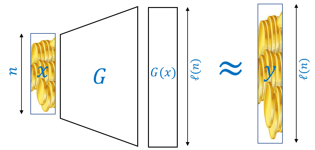
A function \(G:{\{0,1\}}^n\rightarrow{\{0,1\}}^\ell\) is a \((T,\epsilon)\) pseudorandom generator if \(G(U_n) \approx_{T,\epsilon} U_\ell\) where \(U_t\) denotes the uniform distribution on \({\{0,1\}}^t\).
That is, \(G\) is a \((T,\epsilon)\) pseudorandom generator if no circuit of at most \(T\) gates can distinguish with bias better than \(\epsilon\) between the output of \(G\) (on a random input) and a uniformly random string of the same length. Spelling this out fully, this means that for every function \(D:\{0,1\}^\ell \rightarrow \{0,1\}\) computable using at most \(T\) operations,
As we did for the case of encryption, we will typically use asymptotic terms to describe cryptographic pseudorandom generator. We say that \(G\) is simply a pseudorandom generator if it is efficiently computable and it is \((p(n),1/p(n))\)-pseudorandom generator for every polynomial \(p(\cdot)\). In other words, we define pseudorandom generators as follows:
Let \(G:\{0,1\}^* \rightarrow \{0,1\}^*\) be some function computable in polynomial time. We say that \(G\) is a pseudorandom generator with length function \(\ell:\N \rightarrow \N\) (where \(\ell(n)>n\)) if
For every \(x\in \{0,1\}^*\), \(|G(x)| = \ell(|x|)\).
For every polynomial \(p(\cdot)\) and sufficiently large \(n\), if \(D:\{0,1\}^{\ell(n)} \rightarrow \{0,1\}\) is computable by at most \(p(n)\) operations, then
Another way to say it, is that a polynomial-time computable function \(G\) mapping \(n\) bits strings to \(\ell(n)>n\) bit strings is a pseudo-random generator if the two distributions \(G(U_n)\) and \(U_{\ell(n)}\) are computationally indistinguishable.
This definition (as is often the case in cryptography) is a bit long, but the concept of a pseudorandom generator is central to cryptography, and so you should take your time and make sure you understand it. Intuitively, a function \(G\) is a pseudorandom generator if (1) it expands its input (mapping \(n\) bits to \(n+1\) or more) and (2) we cannot distinguish between the output \(G(x)\) for \(x\) a short (i.e., \(n\) bit long) random string, often known as the seed of the pseudorandom generator, and a truly random long (i.e., of length \(\ell(n)\)) string chosen uniformly at random from \(\{0,1\}^{\ell(n)}\).
Note that the requirement that \(\ell>n\) is crucial to make this notion non-trivial, as for \(\ell=n\) the function \(G(x)=x\) clearly satisfies that \(G(U_n)\) is identical to (and hence in particular indistinguishable from) the distribution \(U_n\). (Make sure that you understand this last statement!) However, for \(\ell>n\) this is no longer trivial at all. In particular, if we didn’t restrict the running time of \(Eve\) then no such pseudo-random generator would exist:
Suppose that \(G:{\{0,1\}}^n\rightarrow{\{0,1\}}^{n+1}\). Then there exists an (inefficient) algorithm \(Eve:{\{0,1\}}^{n+1}\rightarrow{\{0,1\}}\) such that \({\mathbb{E}}[ Eve(G(U_n)) ]=1\) but \({\mathbb{E}}[ Eve(U_{n+1})] \leq 1/2\).
On input \(y\in{\{0,1\}}^{n+1}\), consider the algorithm \(Eve\) that goes over all possible \(x\in{\{0,1\}}^n\) and will output \(1\) if and only if \(y=G(x)\) for some \(x\). Clearly \({\mathbb{E}}[ Eve(G(U_n)) ] =1\). However, the set \(S =\{ G(x) : x\in {\{0,1\}}^n \}\) on which Eve outputs \(1\) has size at most \(2^n\), and hence a random \(y{\leftarrow_{\tiny R}} U_{n+1}\) will fall in \(S\) with probability at most \(1/2\).
It is not hard to show that if \(P=\ensuremath{\mathit{NP}}\) then the above algorithm Eve can be made efficient. In particular, at the moment we do not know how to prove the existence of pseudorandom generators. Nevertheless we believe that pseudorandom generators exist and hence we make the following conjecture:
Conjecture (The PRG conjecture): For every \(n\), there exists a pseudorandom generator \(G\) mapping \(n\) bits to \(n+1\) bits.4
As was the case for the cipher conjecture, and any other conjecture, there are two natural questions regarding the PRG conjecture: why should we believe it and why should we care. Fortunately, the answer to the first question is simple: it is known that the cipher conjecture implies the PRG conjecture, and hence if we believe the former we should believe the latter. (The proof is highly non-trivial and we may not get to see it in this course.) As for the second question, we will see that the PRG conjecture implies a great number of useful cryptographic tools, including the cipher conjecture (i.e., the two conjectures are in fact equivalent). We start by showing that once we can get to an output that is one bit longer than the input, we can in fact obtain any polynomial number of bits.
Suppose that the PRG conjecture is true. Then for every polynomial \(t(n)\), there exists a pseudorandom generator mapping \(n\) bits to \(t(n)\) bits.
The proof of this theorem is very similar to the length extension theorem for ciphers, and in fact this theorem can be used to give an alternative proof for the former theorem.
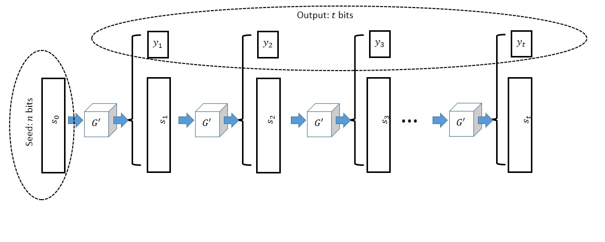
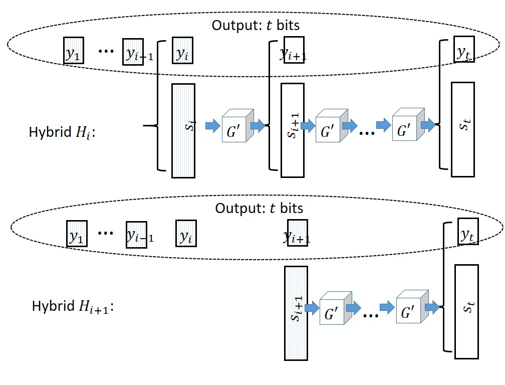
The construction is illustrated in Figure 3.2. We are given a pseudorandom generator \(G'\) mapping \(n\) bits into \(n+1\) bits and need to construct a pseudorandom generator \(G\) mapping \(n\) bits to \(t=t(n)\) bits for some polynomial \(t(\cdot)\). The idea is that we maintain a state of \(n\) bits, which are originally our input seed5 \(s_0\), and at the \(i^{th}\) step we use \(G'\) to map \(s_{i-1}\) to the \(n+1\)-long bit string \((s_i,y_i)\), output \(y_i\) and keep \(s_i\) as our new state. To prove the security of this construction we need to show that the distribution \(G(U_n) = (y_1,\ldots,y_t)\) is computationally indistinguishable from the uniform distribution \(U_t\). As usual, we will use the hybrid argument. For \(i\in\{0,\ldots,t\}\) we define \(H_i\) to be the distribution where the first \(i\) bits chosen uniformly at random, whereas the last \(t-i\) bits are computed as above. Namely, we choose \(s_i\) at random in \(\{0,1\}^n\) and continue the computation of \(y_{i+1},\ldots,y_t\) from the state \(s_i\). Clearly \(H_0=G(U_n)\) and \(H_t=U_t\) and hence by the triangle inequality it suffices to prove that \(H_i \approx H_{i+1}\) for all \(i\in\{0,\ldots,t-1\}\). We illustrate these two hybrids in Figure 3.3.
Now suppose otherwise that there exists some adversary \(Eve\) such that \(\left| \E[Eve(H_i)] - \E[Eve(H_{i+1})] \right| \geq \epsilon\) for some non-negligible \(\epsilon\). From \(Eve\), we will design an adversary \(Eve'\) breaking the security of the pseudorandom generator \(G'\) (see Figure 3.4).
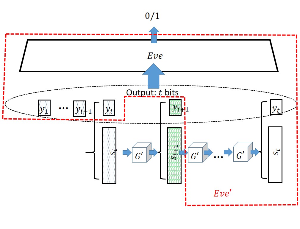
On input a string \(y\) of length \(n+1\), \(Eve'\) will interpret \(y\) as \((s_{i+1},y_{i+1})\) where \(s_{i+1} \in \{0,1\}^n\). She then chooses \(y_1,\ldots,y_i\) randomly and compute \(y_{i+2},\ldots,y_t\) as in our pseudorandom generator’s construction. \(Eve'\) will then feed \((y_1,\ldots,y_t)\) to \(Eve\) and output whatever \(Eve\) does. Clearly, \(Eve'\) is efficient if \(Eve\) is. Moreover, one can see that if \(y\) was random then \(Eve'\) is feeding \(Eve\) with an input distributed according to \(H_{i+1}\) while if \(y\) was of the form \(G(s)\) for a random \(s\) then \(Eve'\) will feed \(Eve\) with an input distributed according to \(H_i\). Hence we get that \(| \E[ Eve'(G'(U_n))] - \E[Eve'(U_{n+1})] | \geq \epsilon\) contradicting the security of \(G'\).
The proof of Theorem 3.4 is indicative of many practical constructions of pseudorandom generators. In many operating systems and programming environments, pseudorandom generators work as follows:
Upon initialization, the system obtains an initial seed of randomness \(x_0 \in \{0,1\}^n\) (where often \(n\) is something like \(128\) or \(256\)).
At the \(t\)-th call to a function such as `rand’ to obtain new randomness, the system uses some underlying pseudorandom generator \(G':\{0,1\}^n \rightarrow \{0,1\}^{n+m}\) to let \(x'\|y = G'(x_{t-1})\), updates \(x_t = x'\) and outputs \(y\).
There are often some additional complications on how to obtain this seed from some “unpredictable” or “high entropy” observations (which can sometimes include network latency, user typing and mouse patterns, and more), and whether the state of the system is periodically “refreshed” using additional observations.
Unpredictability: an alternative approach for proving the length extension theorem
The notion that being random is the same as being “unpredictable”, as discussed at the beginning of this chapter, can be formalized as follows.
An efficiently computable function \(G:\{0,1\}^* \rightarrow \{0,1\}^*\) is unpredictable if, for any \(n\), \(1\le i<\ell(n)\) and polynomially-sized circuit \(P\),
We now show that the condition for a function \(G\) to be unpredictable is equivalent to the condition for it to be a secure PRG. Please make sure you follow the proof, because it is an important theorem, and because it is another example of a canonical cryptographic proof.
Let \(G:\{0,1\}^* \rightarrow \{0,1\}^*\) be a function with length function \(\ell(n)\), then \(G\) is a secure PRG iff it is unpredictable.
For the forward direction, suppose for contradiction that there exists some \(i\) and some circuit \(P\) can predict \(y_i\) given \(y_1,\ldots,y_{i-1}\) with probability \(p\ge \frac12+\epsilon(n)\) for non-negligible \(\epsilon\). Consider the adversary \(Eve\) that, given a string \(y\), runs the circuit \(P\) on \(y_1,\ldots,y_{i-1}\), checks if the output is equal to \(y_i\) and if so output 1.
If \(y=G(x)\) for a uniform \(x\), then \(P\) succeeds with probability \(p\). If \(y\) is uniformly random, then we can imagine that the bit \(y_i\) is generated after \(P\) finished its calculation. The bit \(y_i\) is \(0\) or \(1\) with equal probability, so \(P\) succeeds with probability \(\frac12\). Since \(Eve\) outputs 1 when \(P\) succeeds,
For the backward direction, let \(G\) be an unpredictable function. Let \(H_i\) be the distribution where the first \(i\) bits come from \(G(U_n)\) while the last \(\ell-i\) bits are all random. Notice that \(H_0=U_\ell\) and \(H_\ell=G(U_n)\), so it suffices to show that \(H_{i-1} \approx H_{i}\) for all \(i\).
Suppose \(H_{i-1} \not\approx H_{i}\) for some \(i\), i.e. there exists some \(Eve\) and non-negligible \(\epsilon\) such that
The string \((y_1,\ldots,y_{i-1}, \hat y_i,\ldots,\hat y_\ell)\) has the same distribution as \(H_{i-1}\). However, conditioned on \(\hat y_i=y_i\), the string has distribution equal to \(H_{i}\). Let \(p\) be the probability that \(Eve\) outputs \(1\) if \(\hat y_i=y_i\) and \(q\) be the same probability when \(\hat y_i\neq y_i\), then we get
The definition of unpredictability is useful because many of our candidates for pseudorandom generators appeal to the unpredictability definition in their proofs. For example, the Blum-Blum-Shub generator we will see later in the chapter is proved to be unpredictable if the “quadratic residuosity problem” is hard. It is also nice to know that our intuition at the beginning of the chapter can be formalized.
Stream ciphers
We now show a connection between pseudorandom generators and encryption schemes:
If the PRG conjecture is true then so is the cipher conjecture.
It turns out that the converse direction is also true, and hence these two conjectures are equivalent. We will probably not show the (quite non-trivial) proof of this fact in this course. (We might show a weaker version though.)
Recall that the one time pad is a perfectly secure cipher but its only problem was that to encrypt an \(n+1\) long message it needed an \(n+1\) long bit key. Now using a pseudorandom generator, we can map an \(n\)-bit long key into an \(n+1\)-bit long string that looks random enough that we could use it as a key for the one-time pad. That is, our cipher will look as follows:
and
Just like in the one time pad, \(D_k(E_k(m)) = G(k) \oplus G(k) \oplus m = m\). Moreover, the encryption and decryption algorithms are clearly efficient. We will prove security of this encryption by showing the stronger claim that \(E_{U_n}(m)\approx U_{n+1}\) for any \(m\).
Notice that \(U_{n+1}=U_{n+1}\oplus m\), as we showed in the security of the one-time pad. Suppose that for some non-negligible \(\epsilon=\epsilon(n)>0\) there is an efficient adversary \(Eve'\) such that
Then the adversary \(Eve\) defined as \(Eve(y) = Eve'(y\oplus m)\) would be also efficient. Furthermore, if \(y\) is pseudorandom then \(Eve(y)=Eve'(G(U_n)\oplus m)\) and if \(y\) is uniformly random then \(Eve(y)=Eve'(U_{n+1}\oplus m)\). Then, \(Eve\) can distinguish the two distributions with advantage \(\epsilon\), a contradiction.
If the PRG outputs \(t(n)\) bits instead of \(n+1\) then we automatically get an encryption scheme with \(t(n)\) long message length. In fact, in practice if we use the length extension for PRG’s, we don’t need to decide on the length of messages in advance. Every time we need to encrypt another bit (or another block) \(m_i\) of the message, we run the basic PRG to update our state and obtain some new randomness \(y_i\) that we can XOR with the message and output. Such constructions are known as stream ciphers in the literature. In much of the practical literature, the name stream cipher is used both for the pseudorandom generator itself as well as for the encryption scheme that is obtained by combining it with the one-time pad.
The following is a cute application of pseudorandom generators. Alice and Bob want to toss a fair coin over the phone. They use a pseudorandom generator \(G:\{0,1\}^n\rightarrow\{0,1\}^{3n}\).
- Alice will send \(z\leftarrow_R\{0,1\}^{3n}\) to Bob
- Bob picks \(s\leftarrow_R\{0,1\}^n\) and \(b \leftarrow_R \{0,1\}\). If \(b=0\) then Bob sends \(y=G(s)\) and if \(b=1\) he sends \(y=G(s)\oplus z\). In other words, \(y = G(s) \oplus b\cdot z\) where \(b\cdot z\) is the vector \((b\cdot z_1,\ldots, b\cdot z_{3n})\).
- Alice then picks a random \(b'\leftarrow_R\{0,1\}\) and sends it to Bob.
- Bob sends to Alice the string \(s\) and \(b\). Alice verifies that indeed \(y= G(s) \oplus b \cdot z\). Otherwise Alice aborts.
- The output of the protocol is \(b \oplus b'\).
It can be shown that (assuming the protocol is completed) the output is a random coin, which neither Alice or Bob can control or predict with more than negligible advantage over half. Trying to formalize this and prove it is an excellent exercise. Two main components in the proofs are:
With probability \(1-negl(n)\) over \(z \leftarrow_R \{0,1\}^{3n}\), the sets \(S_0 = \{ G(x) | x\in \{0,1\}^n \}\) and \(S_1 = \{ G(x) \oplus z | x\in \{0,1\}^n \}\) will be disjoint. Hence by choosing \(z\) at random, Alice can ensure that Bob is committed to the choice of \(b\) after sending \(y\).
For every \(z\), both the distribution \(G(U_n)\) and \(G(U_n)\oplus z\) are pseudorandom. This can be shown to imply that no matter what string \(z\) Alice chooses, she cannot predict \(b\) from the string \(y\) sent by Bob with probability better than \(1/2 + negl(n)\). Hence her choice of \(b'\) will be essentially independent of \(b\).
What do pseudorandom generators actually look like?
So far we have made the conjectures that objects such as ciphers and pseudorandom generators exist, without giving any hint as to how they would actually look like. (Though we have examples such as the Caesar cipher, Vigenere, and Enigma of what secure ciphers don’t look like.) As mentioned above, we do not know how to prove that any particular function is a pseudorandom generator. However, there are quite simple candidates (i.e., functions that are conjectured to be secure pseudorandom generators), though care must be taken in constructing them. We now consider candidates for functions that maps \(n\) bits to \(n+1\) bits (or more generally \(n+c\) for some constant \(c\) ) and look at least somewhat “randomish”. As these constructions are typically used as a basic component for obtaining a longer length PRG via the length extension theorem (Theorem 3.4), we will think of these pseudorandom generators as mapping a string \(s\in\{0,1\}^n\) representing the current state into a string \(s’\in\{0,1\}^n\) representing the new state as well as a string \(b\in\{0,1\}^c\) representing the current output. See also Section 6.1 in Katz-Lindell and (for greater depth) Sections 3.6-3.9 in the Boneh-Shoup book.
Attempt 0: The counter generator
To get started, let’s look at an example of an obviously bogus pseudorandom generator. We define the “counter pseudorandom generator” \(G:\{0,1\}^n \rightarrow \{0,1\}^{n+1}\) as follows. \(G(s)=(s',b)\) where \(s' = s + 1 \mod 2^n\) (treating \(s\) and \(s'\) as numbers in \(\{0,\ldots,2^n-1\}\)) and \(b\) is the least significant digit of \(s'\). It’s a great exercise to work out why this is not a secure pseudorandom generator.
You should really pause here and make sure you see why the “counter pseudorandom generator” is not a secure pseudorandom generator. Show that this is true even if we replace the least significant digit by the \(k\)-th digit for every \(0 \leq k < n\).
Attempt 1: The linear checksum / linear feedback shift register (LFSR)
LFSR can be thought of as the “mother” (or maybe more like the sick great-uncle) of all pseudorandom generators. One of the simplest ways to generate a “randomish” extra digit given an \(n\) digit number is to use a checksum - some linear combination of the digits, with a canonical example being the cyclic redundancy check or CRC.6 This motivates the notion of a linear feedback shift register generator (LFSR): if the current state is \(s\in\{0,1\}^n\) then the output is \(f(s)\) where \(f\) is a linear function (modulo 2) and the new state is obtained by right shifting the previous state and putting \(f(s)\) at the leftmost location. That is, \(s'_1 = f(s)\) and \(s'_i = s_{i-1}\) for \(i\in\{2,\ldots,n\}\).
LFSR’s have several good properties- if the function \(f(\cdot)\) is chosen properly then they can have very long periods (i.e., it can take an exponential number of steps until the state repeats itself), though that also holds for the simple “counter” generator we saw above. They also have the property that every individual bit is equal to \(0\) or \(1\) with probability exactly half (the counter generator also shares this property).
A more interesting property is that (if the function is selected properly) every two coordinates are independent from one another. That is, there is some super-polynomial function \(t(n)\) (in fact \(t(n)\) can be exponential in \(n\)) such that if \(\ell \neq \ell' \in \{0,\ldots, t(n) \}\), then if we look at the two random variables corresponding to the \(\ell\)-th and \(\ell'\)-th output of the generator (where randomness is the initial state) then they are distributed like two independent random coins. (This is non-trivial to show, and depends on the choice of \(f\) - it is a challenging but useful exercise to work this out.) The counter generator fails badly at this condition: the least significant bits between two consecutive states always flip.
There is a more general notion of a linear generator where the new state can be any invertible linear transformation of the previous state. That is, we interpret the state \(s\) as an element of \(\Z_q^t\) for some integers \(q,t\),7 and let \(s’=F(s)\) and the output \(b=G(s)\) where \(F:\Z_q^t\rightarrow\Z_q^t\) and \(G:\Z_q^t\rightarrow\Z_q\) are invertible linear transformations (modulo \(q\)). This includes as a special case the linear congruential generator where \(t=1\) and the map \(F(s)\) corresponds to taking \(as \pmod{q}\) where \(a\) is number co-prime to \(q\).
All these generators are unfortunately insecure due to the great bane of cryptography- the Gaussian elimination algorithm which students typically encounter in any linear algebra class.8
There is a polynomial time algorithm to solve \(m\) linear equations in \(n\) variables (or to certify no solution exists) over any ring.
Despite its seeming simplicity and ubiquity, Gaussian elimination (and some generalizations and related algorithms such as Euclid’s extended g.c.d algorithm and the LLL lattice reduction algorithm) has been used time and again to break candidate cryptographic constructions. In particular, if we look at the first \(n\) outputs of a linear generator \(b_1,\ldots,b_n\) then we can write linear equations in the unknown initial state of the form \(f_1(s)=b_1,\ldots,f_n(s)=b_n\) where the \(f_i\)’s are known linear functions. Either those functions are linearly independent, in which case we can solve the equations to get the unique solution for the original state \(s\) and from which point we can predict all outputs of the generator, or they are dependent, which means that we can predict some of the outputs even without recovering the original state. Either way, the generator is \(*\sharp !\)’ed (where \(* \sharp !\) refers to whatever verb you prefer to use when your system is broken). See also this 1977 paper of James Reed.
The above means that it is a bad idea to use a linear checksum as a pseudorandom generator in a cryptographic application, and in fact in any adversarial setting (e.g., one shouldn’t hope that an attacker would not be able to reverse engineer the algorithm9 that computes the control digit of a credit card number). However, that does not mean that there are no legitimate cases where linear generators can be used . In a setting where the application is not adversarial and you have an ability to test if the generator is actually successful, it might be reasonable to use such insecure non-cryptographic generators. They tend to be more efficient (though often not by much) and hence are often the default option in many programming environments such as the C rand() command. (In fact, the real bottleneck in using cryptographic pseudorandom generators is often the generation of entropy for their seed, as discussed in the previous lecture, and not their actual running time.)
From insecurity to security
It is often the case that we want to “fix” a broken cryptographic primitive, such as a pseudorandom generator, to make it secure. At the moment this is still more of an art than a science, but there are some principles that cryptographers have used to try to make this more principled. The main intuition is that there are certain properties of computational problems that make them more amenable to algorithms (i.e., “easier”) and when we want to make the problems useful for cryptography (i.e., “hard”) we often seek variants that don’t possess these properties. The following table illustrates some examples of such properties. (These are not formal statements, but rather is intended to give some intuition )
| Easy | Hard |
|---|---|
| Continuous | Discrete |
| Convex | Non-convex |
| Linear | Non-linear (degree \(\geq 2\)) |
| Noiseless | Noisy |
| Local | Global |
| Shallow | Deep |
| Low degree | High degree |
Many cryptographic constructions can be thought of as trying to transform an easy problem into a hard one by moving from the left to the right column of this table.
The discrete logarithm problem is the discrete version of the continuous real logarithm problem. The learning with errors problem can be thought of as the noisy version of the linear equations problem (or the discrete version of least squares minimization). When constructing block ciphers we often have mixing transformation to ensure that the dependency structure between different bits is global, S-boxes to ensure non-linearity, and many rounds to ensure deep structure and large algebraic degree.
This also works in the other direction. Many algorithmic and machine learning advances work by embedding a discrete problem in a continuous convex one. Some attacks on cryptographic objects can be thought of as trying to recover some of the structure (e.g., by embedding modular arithmetic in the real line or “linearizing” non linear equations).
Attempt 2: Linear Congruential Generators with dropped bits
One approach that is widely used in implementations of pseudorandom generators is to take a linear generator such as the linear congruential generators described above, and use for the output a “chopped” version of the linear function and drop some of the least significant bits. The operation of dropping these bits is non-linear and hence the attack above does not immediately apply. Nevertheless, it turns out this attack can be generalized to handle this case, and hence even with dropped bits Linear Congruential Generators are completely insecure and should be used (if at all) only in applications such as simulations where there is no adversary. Section 3.7.1 in the Boneh-Shoup book describes one attack against such generators that uses the notion of lattice algorithms that we will encounter later in this course in very different contexts.
Successful examples
Let’s now describe some successful (at least per current knowledge) pseudorandom generators:
Case Study 1: Subset Sum Generator
Here is an extremely simple generator that is yet still secure10 as far as we know.
# seed is a list of 40 zero/one values
# output is a 48 bit integer
def subset_sum_gen(seed):
  modulo = 0x1000000
  constants = [
     0x3D6EA1, 0x1E2795, 0xC802C6, 0xBF742A, 0x45FF31,
     0x53A9D4, 0x927F9F, 0x70E09D, 0x56F00A, 0x78B494,
     0x9122E7, 0xAFB10C, 0x18C2C8, 0x8FF050, 0x0239A3,
     0x02E4E0, 0x779B76, 0x1C4FC2, 0x7C5150, 0x81E05E,
     0x154647, 0xB80E68, 0xA042E5, 0xE20269, 0xD3B7F3,
     0xCC5FB9, 0x0BFC55, 0x847AE0, 0x8CFDF8, 0xE304B7,
     0x869ACE, 0xB4CDAB, 0xC8E31F, 0x00EDC7, 0xC50541,
     0x0D6DDD, 0x695A2F, 0xA81062, 0x0123CA, 0xC6C5C3 ]

  # return the modular sum of the constants
  # corresponding to ones in the seed
  return reduce(lambda x,y: (x+y) % modulo,
                map(lambda a,b: a*b, constants,seed))
The seed to this generator is an array seed of 40 bits, with 40 hardwired constants each 48 bits long (these constants were generated at random, but are fixed once and for all, and are not kept secret and hence are not considered part of the secret random seed). The output is simply
This generator is loosely motivated by the “subset sum” computational problem, which is NP hard. However, since NP hardness is a worst case notion of complexity, it does not imply security for pseudorandom generators, which requires hardness of an average case variant. To get some intuition for its security, we can work out why (given that it seems to be linear) we cannot break it by simply using Gaussian elimination.
This is an excellent point for you to stop and try to answer this question on your own.
Given the known constants and known output, figuring out the set of potential seeds can be thought of as solving a single equation in 40 variables. However, this equation is clearly overdetermined, and will have a solution regardless of whether the observed value is indeed an output of the generator, or it is chosen uniformly at random.
More concretely, we can use linear-equation solving to compute (given the known constants \(c_1,\ldots,c_{40} \in \Z_{2^{48}}\) and the output \(y \in \Z_{2^{48}}\)) the linear subspace \(V\) of all vectors \((s_1,\ldots,s_{40}) \in (\Z_{2^{48}})^{40}\) such that \(\sum s_i c_i = y \pmod{2^{48}}\). But, regardless of whether \(y\) was generated at random from \(\Z_{2^{48}}\), or \(y\) was generated as an output of the generator, the subspace \(V\) will always have the same dimension (specifically, since it is formed by a single linear equation over \(40\) variables, the dimension will be \(39\).) To break the generator we seem to need to be able to decide whether this linear subspace \(V \subseteq (\Z_{2^{48}})^{40}\) contains a Boolean vector (i.e., a vector \(s\in \{0,1\}^n\)). Since the condition that a vector is Boolean is not defined by linear equations, we cannot use Gaussian elimination to break the generator. Generally, the task of finding a vector with small coefficients inside a discrete linear subspace is closely related to a classical problem known as finding the shortest vector in a lattice. (See also the short integer solution (SIS) problem.)
Case Study 2: RC4
The following is another example of an extremely simple generator known as RC4 (this stands for Rivest Cipher 4, as Ron Rivest invented this in 1987) and is still fairly widely used today.
def RC4(P,i,j):
    i = (i + 1) % 256
    j = (j + P[i]) % 256
    P[i], P[j] = P[j], P[i]
    return (P,i,j,P[(P[i]+P[j]) % 256])
The function RC4 takes as input the current state P,i,j of the generator and returns the new state together with a single output byte. The state of the generator consists of an array P of 256 bytes, which can be thought of as a permutation of the numbers \(0,\ldots,255\) in the sense that we maintain the invariant that \(\texttt{P}[i]\neq\texttt{P}[j]\) for every \(i\neq j\), and two indices \(i,j \in \{0,\ldots,255\}\). We can consider the initial state as the case where P is a completely random permutation and \(i\) and \(j\) are initialized to zero, although to save on initial seed size, typically RC4 uses some “pseudorandom” way to generate P from a shorter seed as well.
RC4 has extremely efficient software implementations and hence has been widely implemented. However, it has several issues with its security. In particular it was shown by Mantin11 and Shamir that the second bit of RC4 is not random, even if the initialization vector was random. This and other issues led to a practical attack on the 802.11b WiFi protocol, see Section 9.9 in Boneh-Shoup. The initial response to those attacks was to suggest to drop the first 1024 bytes of the output, but by now the attacks have been sufficiently extended that RC4 is simply not considered a secure cipher anymore. The ciphers Salsa and ChaCha, designed by Dan Bernstein, have a similar design to RC4, and are considered secure and deployed in several standard protocols such as TLS, SSH and QUIC, see Section 3.6 in Boneh-Shoup.
Case Study 3: Blum, Blum and Shub
B.B.S., which stands for the authors Blum, Blum and Shub, is a simple generator constructed from a potentially hard problem in number theory.
Let \(N=P\cdot Q\), where \(P,Q\) are primes. (We will generally use \(P,Q\) of size roughly \(n\), where \(n\) is our security parameter, and so use capital letters to emphasize that the magnitude of these numbers is exponential in the security parameter.)
We define \(\ensuremath{\mathit{QR}}_N\) to be the set of quadratic residues modulo \(N\), which are the numbers that have a modular square root. Formally,
This definition extends the concept of “perfect squares” when we are working with standard integers. Notice that each number in \(Y \in \ensuremath{\mathit{QR}}_N\) has at least one square root (number \(X\) such that \(Y = X^2 \mod N\)). We will see later in the course that if \(N = P\cdot Q\) for primes \(P,Q\) then each \(Y\in \ensuremath{\mathit{QR}}_N\) has exactly \(4\) square roots. The B.B.S. generator chooses \(N=P\cdot Q\), where \(P,Q\) are prime and \(P,Q\equiv 3\pmod{4}\). The second condition guarantees that for each \(Y\in \ensuremath{\mathit{QR}}_N\), exactly one of its square roots fall in \(\ensuremath{\mathit{QR}}_N\), and hence the map \(X \mapsto X^2 \mod N\) is one-to-one and onto map from \(\ensuremath{\mathit{QR}}_N\) to itself.
It is defined as follows:
In other words, on input \(X\), \(\ensuremath{\mathit{BBS}}(X)\) outputs \(X^2 \mod N\) and the least significant bit of \(X\). We can think of \(\ensuremath{\mathit{BBS}}\) as a map \(\ensuremath{\mathit{BBS}}:QR_N \rightarrow \ensuremath{\mathit{QR}}_N \times \{0,1\}\) and so it maps a domain into a larger domain. We can also extend it to output \(t\) additional bits, by repeatedly squaring the input, letting \(X_0 = X\), \(X_{i+1} = X_i^2 \mod N\), for \(i=0,\ldots,{t-1}\), and outputting \(X_t\) together with the least significant bits of \(X_0,\ldots,X_{t-1}\). It turns out that assuming that there is no polynomial-time algorithm (where “polynomial-time” means polynomial in the number of bits to represent \(N\), i.e., polynomial in \(\log N\)) to factor randomly chosen integers \(N=P\cdot Q\), for every \(t\) that is polynomial in the number of bits in \(N\), the output of the \(t\)-step \(\ensuremath{\mathit{BBS}}\) generator will be computationally indistinguishable from \(U_{QR_N} \times U_t\) where \(U_{QR_N}\) denotes the uniform distribution over \(\ensuremath{\mathit{QR}}_N\).
The number theory required to show takes a while to develop. However, it is interesting and I recommend the reader to search up this particular generator, see for example this survey by Junod.
Non-constructive existence of pseudorandom generators
We now show that, if we don’t insist on constructivity of pseudorandom generators, then there exists pseudorandom generators with output that are exponentially larger than the input length.
There is some absolute constant \(C\) such that for every \(\epsilon,T\), if \(\ell > C (\log T + \log (1/\epsilon))\) and \(m \leq T\), then there is an \((T,\epsilon)\) pseudorandom generator \(G: \{0,1\}^\ell \rightarrow \{0,1\}^m\).
The proof uses an extremely useful technique known as the “probabilistic method” which is not too hard mathematically but can be confusing at first.12 The idea is to give a “non constructive” proof of existence of the pseudorandom generator \(G\) by showing that if \(G\) was chosen at random, then the probability that it would be a valid \((T,\epsilon)\) pseudorandom generator is positive. In particular this means that there exists a single \(G\) that is a valid \((T,\epsilon)\) pseudorandom generator. The probabilistic method is just a proof technique to demonstrate the existence of such a function. Ultimately, our goal is to show the existence of a deterministic function \(G\) that satisfies the conditions of a \((T, \epsilon)\) PRG.
The above discussion might be rather abstract at this point, but would become clearer after seeing the proof.
Let \(\epsilon,T,\ell,m\) be as in the lemma’s statement. We need to show that there exists a function \(G:\{0,1\}^\ell \rightarrow \{0,1\}^m\) that “fools” every \(T\) line program \(P\) in the sense of Equation 3.1. We will show that this follows from the following claim:
Claim I: For every fixed NAND program / Boolean circuit \(P\), if we pick \(G:\{0,1\}^\ell \rightarrow \{0,1\}^m\) at random then the probability that Equation 3.1 is violated is at most \(2^{-T^2}\).
Before proving Claim I, let us see why it implies Lemma 3.12. We can identify a function \(G:\{0,1\}^\ell \rightarrow \{0,1\}^m\) with its “truth table” or simply the list of evaluations on all its possible \(2^\ell\) inputs. Since each output is an \(m\) bit string, we can also think of \(G\) as a string in \(\{0,1\}^{m\cdot 2^\ell}\). We define \(\mathcal{F}^m_\ell\) to be the set of all functions from \(\{0,1\}^\ell\) to \(\{0,1\}^m\). As discussed above we can identify \(\mathcal{F}_\ell^m\) with \(\{0,1\}^{m\cdot 2^\ell}\) and choosing a random function \(G \sim \mathcal{F}_\ell^m\) corresponds to choosing a random \(m\cdot 2^\ell\)-long bit string.
For every NAND program / Boolean circuit \(P\) let \(B_P\) be the event that, if we choose \(G\) at random from \(\mathcal{F}_\ell^m\) then Equation 3.1 is violated with respect to the program \(P\). It is important to understand what is the sample space that the event \(B_P\) is defined over, namely this event depends on the choice of \(G\) and so \(B_P\) is a subset of \(\mathcal{F}_\ell^m\). An equivalent way to define the event \(B_P\) is that it is the subset of all functions mapping \(\{0,1\}^\ell\) to \(\{0,1\}^m\) that violate Equation 3.1, or in other words: (We’ve replaced here the probability statements in Equation 3.1 with the equivalent sums so as to reduce confusion as to what is the sample space that \(B_P\) is defined over.)
To understand this proof it is crucial that you pause here and see how the definition of \(B_P\) above corresponds to Equation 3.2. This may well take re-reading the above text once or twice, but it is a good exercise at parsing probabilistic statements and learning how to identify the sample space that these statements correspond to.
Now, the number of programs of size \(T\) (or circuits of size \(T\)) is at most \(2^{O(T\log T)}\). Since \(T\log T = o(T^2\)) this means that if Claim I is true, then by the union bound it holds that the probability of the union of \(B_P\) over all NAND programs of at most \(T\) lines is at most \(2^{O(T\log T)}2^{-T^2} < 0.1\) for sufficiently large \(T\). What is important for us about the number \(0.1\) is that it is smaller than \(1\). In particular this means that there exists a single \(G^* \in \mathcal{F}_\ell^m\) such that \(G^*\) does not violate Equation 3.1 with respect to any NAND program of at most \(T\) lines, but that precisely means that \(G^*\) is a \((T,\epsilon)\) pseudorandom generator.
Hence, it suffices to prove Claim I to conclude the proof of Lemma 3.12. Choosing a random \(G: \{0,1\}^\ell \rightarrow \{0,1\}^m\) amounts to choosing \(L=2^\ell\) random strings \(y_0,\ldots,y_{L-1} \in \{0,1\}^m\) and letting \(G(x)=y_x\) (identifying \(\{0,1\}^\ell\) and \([L]\) via the binary representation). Hence the claim amounts to showing that for every fixed function \(P:\{0,1\}^m \rightarrow \{0,1\}\), if \(L > 2^{C (\log T + \log (1/\epsilon))}\) (which by setting \(C>4\), we can ensure is larger than \(10 T^2/\epsilon^2\)) then the probability that is at most \(2^{-T^2}\). ?? ?? follows directly from the Chernoff bound. If we let for every \(i\in [L]\) the random variable \(X_i\) denote \(P(y_i)\), then since \(y_0,\ldots,y_{L-1}\) is chosen independently at random, these are independently and identically distributed random variables with mean \(\E_{y \leftarrow_R \{0,1\}^m}[P(y)]= \Pr_{y\leftarrow_R \{0,1\}^m}[ P(y)=1]\) and hence the probability that they deviate from their expectation by \(\epsilon\) is at most \(2\cdot 2^{-\epsilon^2 L/2}\).
- ↩
Edited and expanded by Richard Xu in Spring 2020.
- ↩
Even lawyers grapple with this question, with a recent example being the debate of whether fantasy football is a game of chance or of skill.
- ↩
In fact such a function must exist in some sense since in the entire history of the world, presumably no sequence of \(100\) fair coin tosses has ever repeated.
- ↩
The name “The PRG conjecture” is non-standard. In the literature this is known as the conjecture of existence of pseudorandom generators. This is a weaker form of “The Optimal PRG Conjecture” presented in my intro to theoretical CS lecture notes since the PRG conjecture only posits the existence of pseudorandom generators with arbitrary polynomial blowup, as opposed to an exponential blowup posited in the optimal PRG conjecture.
- ↩
Because we use a small input to grow a large pseudorandom string, the input to a pseudorandom generator is often known as its seed.
- ↩
CRC are often used to generate a “control digit” to detect mistypes of credit card or social security card number. This has very different goals than its use for pseudorandom generators, though there are some common intuitions behind the two usages.
- ↩
A ring is a set of elements where addition and multiplication are defined and obey the natural rules of associativity and commutativity (though without necessarily having a multiplicative inverse for every element). For every integer \(q\) we define \(\Z_q\) (known as the ring of integers modulo \(q\)) to be the set \(\{0,\ldots,q-1\}\) where addition and multiplication is done modulo \(q\).
- ↩
Despite the name, the algorithm goes at least as far back as the Chinese Jiuzhang Suanshu manuscript, circa 150 B.C.
- ↩
That number is obtained by applying an algorithm of Hans Peter Luhn which applies a simple map to each digit of the card and then sums them up modulo 10.
- ↩
Actually modern computers will be able to break this generator via brute force, but if the length and number of the constants were doubled (or perhaps quadrupled) this should be sufficiently secure, though longer to write down.
- ↩
I typically do not include references in these lecture notes, and leave them to the texts, but I make here an exception because Itsik Mantin was a close friend of mine in grad school.
- ↩
There is a whole (highly recommended) book by Alon and Spencer devoted to this method.
Comments
Comments are posted on the GitHub repository using the utteranc.es app. A GitHub login is required to comment. If you don't want to authorize the app to post on your behalf, you can also comment directly on the GitHub issue for this page.
Compiled on 11/17/2021 22:36:09
Copyright 2021, Boaz Barak.

This work is
licensed under a Creative Commons
Attribution-NonCommercial-NoDerivatives 4.0 International License.
Produced using pandoc and panflute with templates derived from gitbook and bookdown.